4. Land Cover Mapping (Advanced)
In this tutorial we improve the land cover mapping generating probability and uncertantity output per class, as well as an Ensemble Machine Learning approach and a hyperparameter optimization guided by the log_loss metric, suitable for this kind of output. Before continue, please, first execute the Overlay and the Land-Cover Mapping tutorials for the same tile.
This tutorial will map the follow land cover classes using the same covariates provided by the past tutorials:
231: Pastures,
312: Coniferous forest,
321: Natural grasslands,
322: Moors and heathland,
324: Transitional woodland-shrub,
332: Bare rocks,
333: Sparsely vegetated areas,
335: Glaciers and perpetual snow.
First, let’s import the necessary modules
[1]:
# To work with local eumap code
# import sys
# sys.path.append('../../')

import os
import gdal
from pathlib import Path
import pandas as pd
import geopandas as gpd
from eumap.mapper import LandMapper

import warnings
warnings.filterwarnings('ignore')
…and load the overlaid samples for a specific tile:
[2]:
from eumap import datasets

# Tile definition
tile = datasets.pilot.TILES[0]
print(f'Tile: {tile}\n\n')
#datasets.pilot.get_data(tile+'_rasters_gapfilled.tar.gz')

# Folder setup
data_root = datasets.DATA_ROOT_NAME
data_dir = Path(os.getcwd()).joinpath(data_root,tile)

# Reading the samples
fn_points = Path(os.getcwd()).joinpath(data_dir, tile + '_landcover_samples.gpkg')
points = gpd.read_file(fn_points)
points[points.columns[0:12]]
Tile: 10636_switzerland
[2]:
| lucas | survey_date | confidence | tile_id | lc_class | overlay_id | dtm_elevation | dtm_slope | landsat_ard_fall_blue_p25 | landsat_ard_fall_nir_p25 | landsat_ard_fall_green_p25 | landsat_ard_fall_green_p75 | |
|---|---|---|---|---|---|---|---|---|---|---|---|---|
| 0 | False | 2006-06-30T00:00:00 | 85 | 10636 | 321 | 1 | 1948.0 | 36.313705 | 5.0 | 65.0 | 16.0 | 17.0 |
| 1 | False | 2006-06-30T00:00:00 | 85 | 10636 | 321 | 2 | 2209.0 | 7.917305 | 5.0 | 76.0 | 17.0 | 18.0 |
| 2 | False | 2006-06-30T00:00:00 | 85 | 10636 | 321 | 3 | 1990.0 | 32.722038 | 4.0 | 69.0 | 12.0 | 14.0 |
| 3 | False | 2006-06-30T00:00:00 | 85 | 10636 | 322 | 4 | 2142.0 | 49.800537 | 7.0 | 16.0 | 4.0 | 4.0 |
| 4 | False | 2006-06-30T00:00:00 | 85 | 10636 | 332 | 5 | 2420.0 | 27.018671 | 16.0 | 66.0 | 29.0 | 31.0 |
| ... | ... | ... | ... | ... | ... | ... | ... | ... | ... | ... | ... | ... |
| 1119 | False | 2000-06-30T00:00:00 | 85 | 10636 | 312 | 277 | 1729.0 | 16.108473 | 6.0 | 55.0 | 15.0 | 16.0 |
| 1120 | False | 2000-06-30T00:00:00 | 85 | 10636 | 332 | 278 | 2562.0 | 31.661921 | 7.0 | 25.0 | 11.0 | 26.0 |
| 1121 | False | 2000-06-30T00:00:00 | 85 | 10636 | 321 | 279 | 2174.0 | 15.649096 | 5.0 | 77.0 | 15.0 | 17.0 |
| 1122 | False | 2000-06-30T00:00:00 | 85 | 10636 | 333 | 280 | 2368.0 | 21.605083 | 28.0 | 62.0 | 38.0 | 40.0 |
| 1123 | False | 2000-06-30T00:00:00 | 85 | 10636 | 322 | 281 | 900.0 | 27.319332 | 13.0 | 70.0 | 24.0 | 25.0 |
1124 rows × 12 columns
4.1. Probability output
Considering that a probability output provides diferent levels of classification for the target classes, it’s recommended a diferent evaluation metric for the the hyperparameter optimization. Here we choosen log_loss (logistic loss or cross-entropy loss), however you can find more options in scikit-learn - Classification Metrics (hinge_loss, brier_score_loss).
Unlike the F1-Score, a lower log_loss is better for the optimization process, and because of that we will multiply by -1 the returned error.
[3]:
from sklearn.metrics import log_loss

def log_loss_scorer(clf, X, y_true):
    class_labels = clf.classes_
    y_pred_proba = clf.predict_proba(X)
    error = log_loss(y_true, y_pred_proba, labels=class_labels)
    return error * -1
We will use the same classification algorithm, hyperparameter possibilities and cv strategy of the past tutorial:
[4]:
from sklearn.model_selection import GridSearchCV
from sklearn.ensemble import RandomForestClassifier

estimator = RandomForestClassifier(n_estimators=100)

hyperpar = GridSearchCV(
    estimator = estimator,
    scoring = log_loss_scorer,
    param_grid = {
     'min_samples_leaf': [1, 5],
     'max_depth': [5, None],
     'max_features': [0.5]
    }
)
Now let’s create a new instance for the LandMapper class passing one aditional parameter: * pred_method: The predict_proba will change the model output for a lc-class probabilities.
[5]:
feat_col_prfxs = ['landsat', 'dtm', 'night_lights']
target_col = 'lc_class'
weight_col = 'confidence'

min_samples_per_class = 0.05
cv = 5

landmapper_prob = LandMapper(points=points,
                        feat_col_prfxs = feat_col_prfxs,
                        target_col = target_col,
                        estimator = estimator,
                        hyperpar_selection = hyperpar,
                        cv = cv,
                        min_samples_per_class=min_samples_per_class,
                        pred_method='predict_proba',
                        weight_col=weight_col,
                        verbose = True)
[16:18:43] Removing 74 samples (lc_class in [111 122 133 512 221 211 311 132 334]) due min_samples_per_class condition (< 0.05)
[16:18:43] Transforming lc_class:
[16:18:43]  -Original classes: [231. 312. 321. 322. 324. 332. 333. 335.]
[16:18:43]  -Transformed classes: [0 1 2 3 4 5 6 7]
Notice that the original classes were remaped for a sequential class values using LabelEncoder, which can be accessed in the property target_le:
[6]:
landmapper_prob.target_le
[6]:
LabelEncoder()
Time to run (If it’s taking too long try to reduce the hyperparameters possibilities and/or the cv=2):
[7]:
landmapper_prob.train()
[16:18:43] Optimizing hyperparameters for RandomForestClassifier
[16:19:07]  1.04102 (+/-0.06691) from {'max_depth': 5, 'max_features': 0.5, 'min_samples_leaf': 1}
[16:19:07]  1.05511 (+/-0.06881) from {'max_depth': 5, 'max_features': 0.5, 'min_samples_leaf': 5}
[16:19:07]  0.86298 (+/-0.39556) from {'max_depth': None, 'max_features': 0.5, 'min_samples_leaf': 1}
[16:19:07]  0.87060 (+/-0.06458) from {'max_depth': None, 'max_features': 0.5, 'min_samples_leaf': 5}
[16:19:07] Best: -0.86298 using {'max_depth': None, 'max_features': 0.5, 'min_samples_leaf': 1}
[16:19:07] Calculating evaluation metrics
[Parallel(n_jobs=1)]: Using backend SequentialBackend with 1 concurrent workers.
[16:19:18] Training RandomForestClassifier using all samples
[Parallel(n_jobs=1)]: Done 5 out of 5 | elapsed: 8.1s finished
Now let’s take a look in the classification report.
[8]:
print(f'Log loss: {landmapper_prob.eval_metrics["log_loss"]:.3f}\n\n')
print(landmapper_prob.eval_report)
Log loss: 0.814


     log_loss   pr_auc   optimal_prob  optimal_precision  optimal_recall  support

0  0.8454     0.8510   0.3300        0.7576              0.7576         66
1  0.6529     0.7970   0.4400        0.7085              0.7157         199
2  0.8467     0.7925   0.3600        0.7229              0.7229         166
3  1.2766     0.5245   0.3100        0.5517              0.5565         116
4  1.6559     0.3753   0.2700        0.3690              0.3647         84
5  0.7196     0.7917   0.3750        0.7723              0.7723         101
6  0.5459     0.8840   0.4150        0.8079              0.8079         229
7  0.4855     0.9654   0.4890        0.9551              0.9551         89

Total                                                                     1050
Let’s understand this report.
Using the cv result, the LandMapper calculated the log_loss and the pr_auc (area under the precision recall curve) for each class. The pr_auc information was used to choose the best probability value to derive a hard classification output, balancing the precision (producer’s accuracy or the class understimation) and recall (user’s accuracy or the class overestimation), thus minimizing the bias in the land cover area estimation. For more infomation about the precision recall curve access this link.
All the probabilities metrics are available through the prob_metrics property
[9]:
list(landmapper_prob.prob_metrics.keys())
[9]:
['log_loss',
 'pr_auc',
 'support',
 'opti_th',
 'opti_recall',
 'opti_precision',
 'curv_recall',
 'curv_precision',
 'curv_th']
…and it’s possible to use the raw cv results to derive other evaluation metrics as hinge_loss:
[10]:
from sklearn import preprocessing, metrics

# Tranform the target classes in probability values
lb = preprocessing.LabelBinarizer()
targ_prob = lb.fit_transform(landmapper_prob.target)
n_classes = len(lb.classes_)

# Brier loss calculation for each class
print('Brier loss:')
for c in range(0,n_classes):
    brier_loss = metrics.brier_score_loss(targ_prob[:,c], landmapper_prob.eval_pred[:,c])
    print(f' - {lb.classes_[c]:.0f}: {brier_loss * 100:.3f}%')
Brier loss:
 - 0: 2.515%
 - 1: 7.276%
 - 2: 6.671%
 - 3: 6.822%
 - 4: 6.071%
 - 5: 3.559%
 - 6: 6.494%
 - 7: 0.733%
4.2. EML (Emsemble Machine Learning) and uncertainties
Up until now only one estimator was used to produce the land cover maps. Even considering that the Random Forest is a emsemble of DecisionTreeClassifier, the trees growth uses the same rationale to train a weak estimator considering different proportions of the full dataset (Bagging approach). A combination of the Random Forest with other estimators will produce multiple predicted values, produced by different approachs/algorithms that consequently splits the feature space in a diferent way, allowing the derivation of a final probability and a uncertanty estimative, based in the standard deviation of all predicted probabilties
To do it, let’s first create our traditional estimator:
[11]:
estimator_rf = RandomForestClassifier(n_jobs=-1, n_estimators=85)

hyperpar_rf = GridSearchCV(
    estimator = estimator_rf,
    scoring = log_loss_scorer,
    param_grid = {
     'max_depth': [5, None],
     'max_features': [0.5, None]
    }
)
In addition to Random Forest we will use the XGBoost
[12]:
import xgboost as xgb
estimator_bgtree = xgb.XGBClassifier(n_jobs=-1, n_estimators=28, objective='multi:softmax',
                                     use_label_encoder=False, eval_metric='mlogloss', booster='gbtree')

hyperpar_bgtree = GridSearchCV(
    estimator = estimator_bgtree,
    scoring = log_loss_scorer,
    param_grid = {
     'eta': [0.001, 0.9],
     'alpha': [0, 10]
    }
)
…and a regular ANN (Artificial Neural Network) through KerasClassifier:
[13]:
from sklearn.pipeline import Pipeline
from sklearn.preprocessing import StandardScaler
from tensorflow.keras.wrappers.scikit_learn import KerasClassifier
from eumap.mapper import build_ann

input_shape = 87
n_classes = 8
estimator_ann = Pipeline([
    ('standardize', StandardScaler()),
    ('estimator', KerasClassifier(build_ann, input_shape=input_shape, output_shape=n_classes, \
            epochs=5, batch_size=64, learning_rate = 0.0005, \
            dropout_rate=0.15, n_layers = 4, n_neurons=64, shuffle=True, verbose=False))
])

hyperpar_ann = GridSearchCV(
    estimator = estimator_ann,
    scoring = log_loss_scorer,
    param_grid = {
     'estimator__dropout_rate': [0, 0.15],
     'estimator__n_layers': [2, 4]
    }
)
It’s important to choose modern estimators able to produce results equally accurate and comparable to the Random Forest, otherwise they could produce a poor classification results at end.
The three predicted probabilities will be combined by a meta-estimator, which will receive as n_estimator * n_classes covariates/features as input and produce the final output:
[14]:
from sklearn.linear_model import LogisticRegression

meta_estimator = LogisticRegression(solver='saga', multi_class='multinomial')

hyperpar_meta = GridSearchCV(
    estimator = meta_estimator,
    scoring = log_loss_scorer,
    param_grid = {
        'fit_intercept': [False, True],
        'C': [0.5, 1]
    }
)
To pass the three estimators and their respective hyperparameter optimization critereas we will use estimator_list and hyperpar_selection_list, using the same element orders for both:
[15]:
feat_col_prfxs = ['landsat', 'dtm', 'night_lights']
target_col = 'lc_class'
weight_col = 'confidence'

min_samples_per_class = 0.05
cv = 2

estimator_list = [estimator_rf, estimator_bgtree, estimator_ann]
hyperpar_selection_list = [hyperpar_rf, hyperpar_bgtree, hyperpar_ann]

landmapper_eml = LandMapper(points=fn_points,
                        feat_col_prfxs = feat_col_prfxs,
                        target_col = target_col,
                        estimator_list = estimator_list,
                        meta_estimator = meta_estimator,
                        hyperpar_selection_list = hyperpar_selection_list,
                        hyperpar_selection_meta = hyperpar_meta,
                        min_samples_per_class = min_samples_per_class,
                        cv = cv,
                        verbose = True)
[16:19:20] Removing 74 samples (lc_class in [111 122 133 512 221 211 311 132 334]) due min_samples_per_class condition (< 0.05)
[16:19:20] Transforming lc_class:
[16:19:20]  -Original classes: [231. 312. 321. 322. 324. 332. 333. 335.]
[16:19:20]  -Transformed classes: [0 1 2 3 4 5 6 7]
Time to train our EML estimator:
[16]:
landmapper_eml.train()
[16:19:20] Optimizing hyperparameters for RandomForestClassifier
[16:19:25]  1.05089 (+/-0.00010) from {'max_depth': 5, 'max_features': 0.5}
[16:19:25]  1.02881 (+/-0.01823) from {'max_depth': 5, 'max_features': None}
[16:19:25]  0.81177 (+/-0.02959) from {'max_depth': None, 'max_features': 0.5}
[16:19:25]  0.85910 (+/-0.12577) from {'max_depth': None, 'max_features': None}
[16:19:25] Best: -0.81177 using {'max_depth': None, 'max_features': 0.5}
[16:19:25] Optimizing hyperparameters for XGBClassifier
[16:19:29]  2.03720 (+/-0.00099) from {'alpha': 0, 'eta': 0.001}
[16:19:29]  1.02404 (+/-0.25651) from {'alpha': 0, 'eta': 0.9}
[16:19:29]  2.05202 (+/-0.00139) from {'alpha': 10, 'eta': 0.001}
[16:19:29]  1.15856 (+/-0.07229) from {'alpha': 10, 'eta': 0.9}
[16:19:29] Best: -1.02404 using {'alpha': 0, 'eta': 0.9}
[16:19:29] Optimizing hyperparameters for Pipeline
[16:19:52]  1.79155 (+/-0.01856) from {'estimator__dropout_rate': 0, 'estimator__n_layers': 2}
[16:19:52]  1.93725 (+/-0.06209) from {'estimator__dropout_rate': 0, 'estimator__n_layers': 4}
[16:19:52]  1.74485 (+/-0.12721) from {'estimator__dropout_rate': 0.15, 'estimator__n_layers': 2}
[16:19:52]  1.85103 (+/-0.06167) from {'estimator__dropout_rate': 0.15, 'estimator__n_layers': 4}
[16:19:52] Best: -1.74485 using {'estimator__dropout_rate': 0.15, 'estimator__n_layers': 2}
[16:19:52] Calculating meta-features
[Parallel(n_jobs=1)]: Using backend SequentialBackend with 1 concurrent workers.
[Parallel(n_jobs=1)]: Done   2 out of   2 | elapsed:    0.7s finished
[Parallel(n_jobs=1)]: Using backend SequentialBackend with 1 concurrent workers.
[Parallel(n_jobs=1)]: Done   2 out of   2 | elapsed:    1.3s finished
[Parallel(n_jobs=1)]: Using backend SequentialBackend with 1 concurrent workers.
[16:19:58]  Meta-features shape: (1050, 24)
[16:19:58] Optimizing hyperparameters for LogisticRegression
[Parallel(n_jobs=1)]: Done 2 out of 2 | elapsed: 4.4s finished
[16:19:59]  0.86881 (+/-0.07034) from {'C': 0.5, 'fit_intercept': False}
[16:19:59]  0.86736 (+/-0.06701) from {'C': 0.5, 'fit_intercept': True}
[16:19:59]  0.84879 (+/-0.07620) from {'C': 1, 'fit_intercept': False}
[16:19:59]  0.84782 (+/-0.07341) from {'C': 1, 'fit_intercept': True}
[16:19:59] Best: -0.84782 using {'C': 1, 'fit_intercept': True}
[16:19:59] Calculating evaluation metrics
[16:19:59] Training RandomForestClassifier using all samples
[Parallel(n_jobs=1)]: Using backend SequentialBackend with 1 concurrent workers.
[Parallel(n_jobs=1)]: Done   2 out of   2 | elapsed:    0.1s finished
[16:19:59] Training XGBClassifier using all samples
[16:20:00] Training Pipeline using all samples
[16:20:02] Training meta-estimator using all samples
…and about the classification report?
[17]:
print(f'Log loss: {landmapper_eml.eval_metrics["log_loss"]:.3f}\n\n')
print(landmapper_eml.eval_report)
Log loss: 0.848


     log_loss   pr_auc   optimal_prob  optimal_precision  optimal_recall  support

0  0.8513     0.8262   0.3686        0.7576              0.7576         66
1  0.7929     0.7601   0.4908        0.6884              0.6884         199
2  0.8432     0.7756   0.3289        0.7229              0.7229         166
3  1.4399     0.4948   0.2617        0.5000              0.5000         116
4  1.8697     0.2404   0.2036        0.2738              0.2738         84
5  0.7568     0.7986   0.3566        0.7525              0.7525         101
6  0.4965     0.8880   0.3970        0.8122              0.8122         229
7  0.2479     0.9820   0.4704        0.9438              0.9438         89

Total                                                                     1050
Now we are ready to run the predictions passing the follow parameters: * dirs_layers: a list containing diferent folders that store the same raster layers used in the spacetive overlay and training phase, * fn_output: the file path to write the model output as geotiff.
[18]:
dir_timeless_layers = os.path.join(data_dir, 'timeless')
dir_2000_layers = os.path.join(data_dir, '2000')

dirs_layers = [dir_2000_layers, dir_timeless_layers]
fn_output = os.path.join(data_dir, 'land_cover_eml_2000.tif')

output_fn_files = landmapper_eml.predict(dirs_layers=dirs_layers, fn_output=fn_output, allow_additional_layers=True)

print('Output files:')
for output_fn_file in output_fn_files:
    print(f' - {Path(output_fn_file).name}')
[16:20:02] Reading 87 raster files using 4 workers
[16:20:08] Executing RandomForestClassifier
[16:20:11] RandomForestClassifier prediction time: 2.66 segs
[16:20:11] Executing XGBClassifier
[16:20:11] XGBClassifier prediction time: 0.44 segs
[16:20:11] Executing Pipeline
[16:20:11] batch_size=500000
[16:20:55] Pipeline prediction time: 43.22 segs
[16:20:55] Executing LogisticRegression
[16:20:56] LogisticRegression prediction time: 1.33 segs
Output files:
 - land_cover_eml_2000_b1.tif
 - land_cover_eml_2000_b2.tif
 - land_cover_eml_2000_b3.tif
 - land_cover_eml_2000_b4.tif
 - land_cover_eml_2000_b5.tif
 - land_cover_eml_2000_b6.tif
 - land_cover_eml_2000_b7.tif
 - land_cover_eml_2000_b8.tif
 - land_cover_eml_2000_hcl.tif
 - land_cover_eml_2000_hcl_prob.tif
 - land_cover_eml_2000_uncertainty_b1.tif
 - land_cover_eml_2000_uncertainty_b2.tif
 - land_cover_eml_2000_uncertainty_b3.tif
 - land_cover_eml_2000_uncertainty_b4.tif
 - land_cover_eml_2000_uncertainty_b5.tif
 - land_cover_eml_2000_uncertainty_b6.tif
 - land_cover_eml_2000_uncertainty_b7.tif
 - land_cover_eml_2000_uncertainty_b8.tif
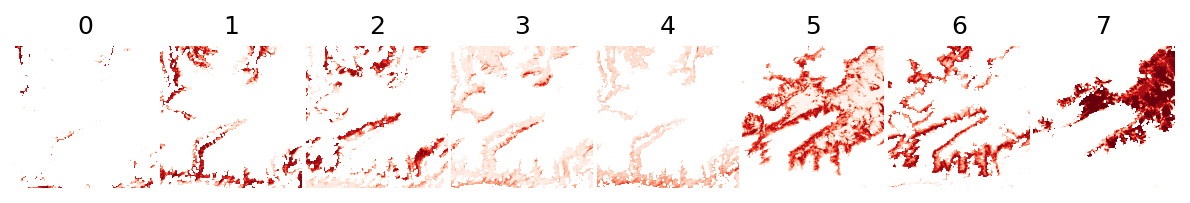
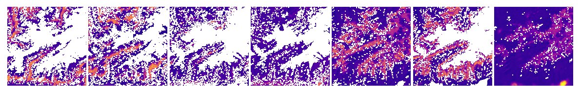
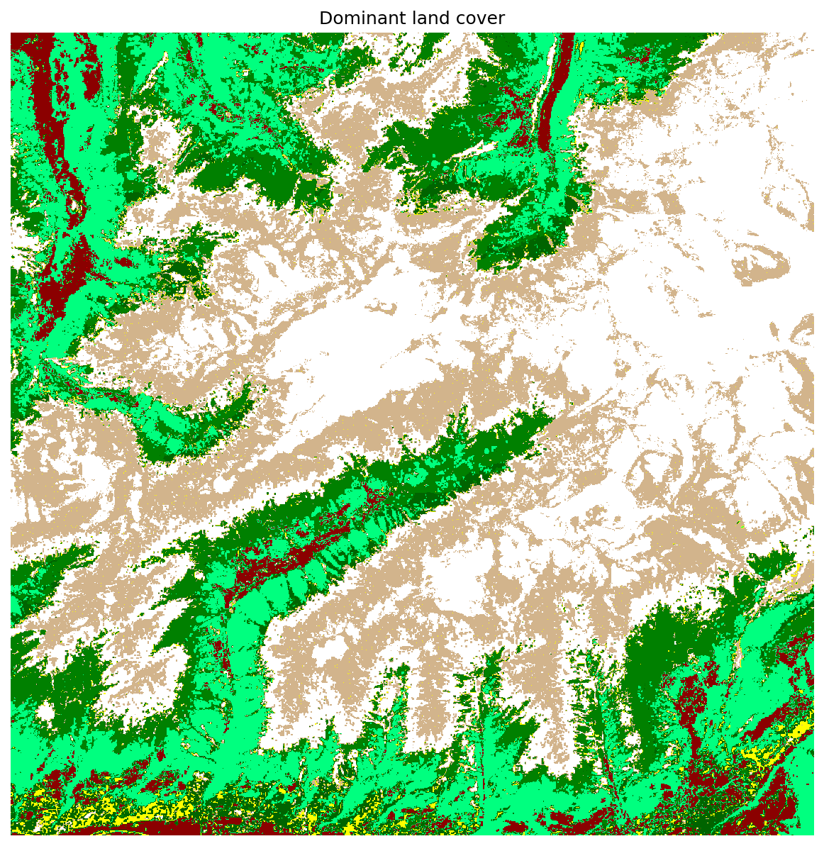
Let’s understand the output files: * Probabilities/Uncertainties: For each land cover class was generated a raster file with the predicted probability/uncertainty. The output filename is equal defined by {fn_output}_b{target_class_transformed}.tif * Dominant/Hard classes: The dominant/hard class file (*hcl.tif) was generated assuming the highest probability value as final class. The *hcl_prob.tif presents the probability of the chosen land cover class.
It’s possible access the original and transformed values in the property target_classes:
[19]:
labels = [
    '231: Pastures',
    '312: Coniferous forest',
    '321: Natural grasslands',
    '322: Moors and heathland',
    '324: Transitional woodland-shrub',
    '332: Bare rocks',
    '333: Sparsely vegetated areas',
    '335: Glaciers and perpetual snow'
]

pd.DataFrame({
    'Label':labels,
    'Original': landmapper_eml.target_classes['original'],
    'Transformed': landmapper_eml.target_classes['transformed']
})
[19]:
| Label | Original | Transformed | |
|---|---|---|---|
| 0 | 231: Pastures | 231.0 | 0 |
| 1 | 312: Coniferous forest | 312.0 | 1 |
| 2 | 321: Natural grasslands | 321.0 | 2 |
| 3 | 322: Moors and heathland | 322.0 | 3 |
| 4 | 324: Transitional woodland-shrub | 324.0 | 4 |
| 5 | 332: Bare rocks | 332.0 | 5 |
| 6 | 333: Sparsely vegetated areas | 333.0 | 6 |
| 7 | 335: Glaciers and perpetual snow | 335.0 | 7 |
Let’s see the the probability and uncertainty outputs:
[20]:
import numpy as np
from eumap.plotter import plot_rasters

lc_classes = [ int(c) for c in landmapper_eml.target_classes['transformed']]

plot_rasters(*output_fn_files[0:8], cmaps='Reds', titles=lc_classes)
plot_rasters(*output_fn_files[11:19], cmaps='plasma')
…and the dominant land cover:
[21]:
from eumap.plotter import plot_rasters
import numpy as np
from matplotlib.colors import ListedColormap

lc_classes = landmapper_eml.target_classes['original']
pixel_values = landmapper_eml.target_classes['transformed']
colors = ListedColormap(["red", "darkred", "springgreen", "green", "darkgreen", "yellow", "tan", "white"])

print("Mapped land cover classes")
for l, p, c in zip(lc_classes, pixel_values, colors.colors):
    print(f' - {l:.0f} => pixel value {p} ({c})')

plot_rasters(output_fn_files[8], cmaps = colors, titles = 'Dominant land cover')
Mapped land cover classes
 - 231 => pixel value 0 (red)
 - 312 => pixel value 1 (darkred)
 - 321 => pixel value 2 (springgreen)
 - 322 => pixel value 3 (green)
 - 324 => pixel value 4 (darkgreen)
 - 332 => pixel value 5 (yellow)
 - 333 => pixel value 6 (tan)
 - 335 => pixel value 7 (white)
Time to predict multiple years creating a list of dirs_layers and fn_output and passing to the method predict_multi, which will perform this task in parallel:
[22]:
dir_timeless_layers = os.path.join(data_dir, 'timeless')

dirs_layers_list = []
fn_output_list = []

for year in range(2000, 2003):
    dir_time_layers = os.path.join(data_dir, str(year))
    dirs_layers = [dir_time_layers, dir_timeless_layers]
    fn_result = os.path.join(data_dir, f'land_cover_eml_{year}.tif')

    dirs_layers_list.append(dirs_layers)
    fn_output_list.append(fn_result)

output_fn_files = landmapper_eml.predict_multi(dirs_layers_list=dirs_layers_list, fn_output_list=fn_output_list, allow_additional_layers=True)

print('Output files:')
for output_fn_file in output_fn_files:
    print(f' - {Path(output_fn_file).name}')
[16:21:00] Reading 87 raster files using 5 workers
[16:21:06] 1) Reading time: 5.78 segs
[16:21:06] 1) Predicting 1000000 pixels
[16:21:06] Reading 87 raster files using 5 workers
[16:21:06] Executing RandomForestClassifier
[16:21:09] RandomForestClassifier prediction time: 2.90 segs
[16:21:09] Executing XGBClassifier
[16:21:10] XGBClassifier prediction time: 0.63 segs
[16:21:10] Executing Pipeline
[16:21:10] batch_size=500000
[16:21:13] 2) Reading time: 6.72 segs
[16:21:13] Reading 87 raster files using 5 workers
[16:21:19] 3) Reading time: 5.90 segs
[16:21:51] Pipeline prediction time: 41.49 segs
[16:21:51] Executing LogisticRegression
[16:21:53] LogisticRegression prediction time: 1.46 segs
[16:21:53] 1) Predicting time: 46.53 segs
[16:21:53] 2) Predicting 1000000 pixels
[16:21:53] Executing RandomForestClassifier
[16:21:54] 1) Saving time: 1.19 segs
[16:21:56] RandomForestClassifier prediction time: 2.94 segs
[16:21:56] Executing XGBClassifier
[16:21:56] XGBClassifier prediction time: 0.39 segs
[16:21:56] Executing Pipeline
[16:21:56] batch_size=500000
[16:22:39] Pipeline prediction time: 42.70 segs
[16:22:39] Executing LogisticRegression
[16:22:41] LogisticRegression prediction time: 1.45 segs
[16:22:41] 2) Predicting time: 47.50 segs
[16:22:41] 3) Predicting 1000000 pixels
[16:22:41] Executing RandomForestClassifier
[16:22:42] 2) Saving time: 1.05 segs
[16:22:44] RandomForestClassifier prediction time: 2.66 segs
[16:22:44] Executing XGBClassifier
[16:22:44] XGBClassifier prediction time: 0.38 segs
[16:22:44] Executing Pipeline
[16:22:44] batch_size=500000
[16:23:26] Pipeline prediction time: 42.09 segs
[16:23:26] Executing LogisticRegression
[16:23:28] LogisticRegression prediction time: 1.36 segs
[16:23:28] 3) Predicting time: 46.54 segs
[16:23:28] 3) Saving time: 0.59 segs
Output files:
 - land_cover_eml_2000_b1.tif
 - land_cover_eml_2000_b2.tif
 - land_cover_eml_2000_b3.tif
 - land_cover_eml_2000_b4.tif
 - land_cover_eml_2000_b5.tif
 - land_cover_eml_2000_b6.tif
 - land_cover_eml_2000_b7.tif
 - land_cover_eml_2000_b8.tif
 - land_cover_eml_2000_hcl.tif
 - land_cover_eml_2000_hcl_prob.tif
 - land_cover_eml_2000_uncertainty_b1.tif
 - land_cover_eml_2000_uncertainty_b2.tif
 - land_cover_eml_2000_uncertainty_b3.tif
 - land_cover_eml_2000_uncertainty_b4.tif
 - land_cover_eml_2000_uncertainty_b5.tif
 - land_cover_eml_2000_uncertainty_b6.tif
 - land_cover_eml_2000_uncertainty_b7.tif
 - land_cover_eml_2000_uncertainty_b8.tif
 - land_cover_eml_2001_b1.tif
 - land_cover_eml_2001_b2.tif
 - land_cover_eml_2001_b3.tif
 - land_cover_eml_2001_b4.tif
 - land_cover_eml_2001_b5.tif
 - land_cover_eml_2001_b6.tif
 - land_cover_eml_2001_b7.tif
 - land_cover_eml_2001_b8.tif
 - land_cover_eml_2001_hcl.tif
 - land_cover_eml_2001_hcl_prob.tif
 - land_cover_eml_2001_uncertainty_b1.tif
 - land_cover_eml_2001_uncertainty_b2.tif
 - land_cover_eml_2001_uncertainty_b3.tif
 - land_cover_eml_2001_uncertainty_b4.tif
 - land_cover_eml_2001_uncertainty_b5.tif
 - land_cover_eml_2001_uncertainty_b6.tif
 - land_cover_eml_2001_uncertainty_b7.tif
 - land_cover_eml_2001_uncertainty_b8.tif
 - land_cover_eml_2002_b1.tif
 - land_cover_eml_2002_b2.tif
 - land_cover_eml_2002_b3.tif
 - land_cover_eml_2002_b4.tif
 - land_cover_eml_2002_b5.tif
 - land_cover_eml_2002_b6.tif
 - land_cover_eml_2002_b7.tif
 - land_cover_eml_2002_b8.tif
 - land_cover_eml_2002_hcl.tif
 - land_cover_eml_2002_hcl_prob.tif
 - land_cover_eml_2002_uncertainty_b1.tif
 - land_cover_eml_2002_uncertainty_b2.tif
 - land_cover_eml_2002_uncertainty_b3.tif
 - land_cover_eml_2002_uncertainty_b4.tif
 - land_cover_eml_2002_uncertainty_b5.tif
 - land_cover_eml_2002_uncertainty_b6.tif
 - land_cover_eml_2002_uncertainty_b7.tif
 - land_cover_eml_2002_uncertainty_b8.tif
The LandMapper also supports a eager prediction strategy that reads all the years, run the predictions for all the data at once and write the output files:
[23]:
from eumap.mapper import PredictionStrategyType

pred_strategy_type = PredictionStrategyType.Eager
output_fn_files = landmapper_eml.predict_multi(dirs_layers_list=dirs_layers_list, fn_output_list=fn_output_list, \
                                               allow_additional_layers=True, prediction_strategy_type=pred_strategy_type)

print('Output files:')
for output_fn_file in output_fn_files:
    print(f' - {Path(output_fn_file).name}')
[16:23:29] Reading 87 raster files using 5 workers
[16:23:29] Reading 87 raster files using 5 workers
[16:23:29] Reading 87 raster files using 5 workers
[16:23:36] 2) Reading time: 7.37 segs
[16:23:36] 1) Reading time: 7.51 segs
[16:23:37] 3) Reading time: 8.33 segs
[16:23:37] 3) Predicting 3000000 pixels
[16:23:38] Executing RandomForestClassifier
[16:23:45] RandomForestClassifier prediction time: 7.27 segs
[16:23:45] Executing XGBClassifier
[16:23:46] XGBClassifier prediction time: 1.17 segs
[16:23:46] Executing Pipeline
[16:23:46] batch_size=1500000
[16:25:55] Pipeline prediction time: 128.80 segs
[16:25:55] Executing LogisticRegression
[16:25:59] LogisticRegression prediction time: 4.02 segs
[16:25:59] 3) Predicting time: 141.39 segs
[16:26:02] 2) Saving time: 2.22 segs
[16:26:02] 3) Saving time: 2.28 segs
[16:26:02] 1) Saving time: 2.35 segs
Output files:
 - land_cover_eml_2000_b1.tif
 - land_cover_eml_2000_b2.tif
 - land_cover_eml_2000_b3.tif
 - land_cover_eml_2000_b4.tif
 - land_cover_eml_2000_b5.tif
 - land_cover_eml_2000_b6.tif
 - land_cover_eml_2000_b7.tif
 - land_cover_eml_2000_b8.tif
 - land_cover_eml_2000_hcl.tif
 - land_cover_eml_2000_hcl_prob.tif
 - land_cover_eml_2000_uncertainty_b1.tif
 - land_cover_eml_2000_uncertainty_b2.tif
 - land_cover_eml_2000_uncertainty_b3.tif
 - land_cover_eml_2000_uncertainty_b4.tif
 - land_cover_eml_2000_uncertainty_b5.tif
 - land_cover_eml_2000_uncertainty_b6.tif
 - land_cover_eml_2000_uncertainty_b7.tif
 - land_cover_eml_2000_uncertainty_b8.tif
 - land_cover_eml_2001_b1.tif
 - land_cover_eml_2001_b2.tif
 - land_cover_eml_2001_b3.tif
 - land_cover_eml_2001_b4.tif
 - land_cover_eml_2001_b5.tif
 - land_cover_eml_2001_b6.tif
 - land_cover_eml_2001_b7.tif
 - land_cover_eml_2001_b8.tif
 - land_cover_eml_2001_hcl.tif
 - land_cover_eml_2001_hcl_prob.tif
 - land_cover_eml_2001_uncertainty_b1.tif
 - land_cover_eml_2001_uncertainty_b2.tif
 - land_cover_eml_2001_uncertainty_b3.tif
 - land_cover_eml_2001_uncertainty_b4.tif
 - land_cover_eml_2001_uncertainty_b5.tif
 - land_cover_eml_2001_uncertainty_b6.tif
 - land_cover_eml_2001_uncertainty_b7.tif
 - land_cover_eml_2001_uncertainty_b8.tif
 - land_cover_eml_2002_b1.tif
 - land_cover_eml_2002_b2.tif
 - land_cover_eml_2002_b3.tif
 - land_cover_eml_2002_b4.tif
 - land_cover_eml_2002_b5.tif
 - land_cover_eml_2002_b6.tif
 - land_cover_eml_2002_b7.tif
 - land_cover_eml_2002_b8.tif
 - land_cover_eml_2002_hcl.tif
 - land_cover_eml_2002_hcl_prob.tif
 - land_cover_eml_2002_uncertainty_b1.tif
 - land_cover_eml_2002_uncertainty_b2.tif
 - land_cover_eml_2002_uncertainty_b3.tif
 - land_cover_eml_2002_uncertainty_b4.tif
 - land_cover_eml_2002_uncertainty_b5.tif
 - land_cover_eml_2002_uncertainty_b6.tif
 - land_cover_eml_2002_uncertainty_b7.tif
 - land_cover_eml_2002_uncertainty_b8.tif
4.3. Feature Selection
The LandMapper is fully compatible with scikit-learn, supporting any BaseEstimator and Pipeline implementations.
To demonstrate it, we will develop from scratch a simple random feature selection strategy, which will randomly reduce the number of input features before the training step.
[24]:
from numpy.random import default_rng
from sklearn.base import BaseEstimator, TransformerMixin

class RandomFeatureSelector(TransformerMixin, BaseEstimator):

    def __init__(self, n_features = 10, seed = 0):
        self.n_features = n_features
        self.rng = default_rng()
        self.seed = seed

    def fit(self, X, y):
        n_features = X.shape[1]
        self.rand_features = self.rng.choice(n_features, size=self.n_features, replace=False)
        return self

    def transform(self, X):
        return X[:,self.rand_features]
Now let’s define the expected number of features (there are 87 features in total), changing the input seed to produce diferent subsets. The passthrough will indicate to the pipeline just move foward to the next step.
[25]:
feature_sel = [
    RandomFeatureSelector(n_features=60, seed = 0),
    RandomFeatureSelector(n_features=70, seed = 0),
    RandomFeatureSelector(n_features=80, seed = 0),
    RandomFeatureSelector(n_features=60, seed = 1),
    RandomFeatureSelector(n_features=70, seed = 1),
    RandomFeatureSelector(n_features=80, seed = 1),
    'passthrough'
]
This time we will define our estimators as pipelines, indicating the feature_sel step before them
[26]:
estimator_rf = Pipeline([
    ('feature_sel', 'passthrough'),
    ('estimator', RandomForestClassifier(n_jobs=-1, max_depth=None,  n_estimators=85))
])

estimator_bgtree = Pipeline([
    ('feature_sel', 'passthrough'),
    ('estimator', xgb.XGBClassifier(n_jobs=-1, n_estimators=28, use_label_encoder=False, objective='multi:softmax', eval_metric='mlogloss', booster='gbtree'))
])

estimator_ann = Pipeline([
    ('feature_sel', 'passthrough'),
    ('standardize', StandardScaler()),
    ('estimator', KerasClassifier(build_ann, input_shape=input_shape, output_shape=n_classes, \
        epochs=5, batch_size=64, learning_rate = 0.0005, \
        dropout_rate=0.15, n_layers = 4, n_neurons=64, shuffle=True, verbose=False))
])
…and adding the feature_sel possibilities as a property in our hyperparameter optimization class (GridSearchCV):
[27]:
hyperpar_rf = GridSearchCV(
    estimator = estimator_rf,
    scoring = log_loss_scorer,
    verbose = True,
    param_grid = {
     'feature_sel': feature_sel,
     'estimator__max_depth': [5, None],
     'estimator__max_features': [0.5, None]
    }
)

hyperpar_bgtree = GridSearchCV(
    estimator = estimator_bgtree,
    scoring = log_loss_scorer,
    verbose = True,
    param_grid = {
     'feature_sel': feature_sel,
     'estimator__eta': [0.001, 0.9],
     'estimator__alpha': [0, 10]
    }
)

hyperpar_ann = GridSearchCV(
    estimator = estimator_ann,
    scoring = log_loss_scorer,
    verbose = True,
    param_grid = {
     'feature_sel': feature_sel,
     'estimator__dropout_rate': [0, 0.15],
     'estimator__n_layers': [2, 4]
    }
)
Let’s keep the same meta-estimator
[28]:
meta_estimator = LogisticRegression(solver='saga', multi_class='multinomial', C=1, fit_intercept=True)
… and LandMapper parameters:
[29]:
feat_col_prfxs = ['landsat', 'dtm', 'night_lights']
target_col = 'lc_class'
weight_col = 'confidence'

min_samples_per_class = 0.05
cv = 2

landmapper_feat_sel = LandMapper(points=fn_points,
                                feat_col_prfxs = feat_col_prfxs,
                                target_col = target_col,
                                estimator_list = [estimator_rf, estimator_bgtree, estimator_ann],
                                hyperpar_selection_list = [hyperpar_rf, hyperpar_bgtree, hyperpar_ann],
                                meta_estimator = meta_estimator,
                                min_samples_per_class = min_samples_per_class,
                                cv = cv,
                                pred_method='predict_proba',
                                verbose = True)

landmapper_feat_sel.train()
[16:26:03] Removing 74 samples (lc_class in [111 122 133 512 221 211 311 132 334]) due min_samples_per_class condition (< 0.05)
[16:26:03] Transforming lc_class:
[16:26:03]  -Original classes: [231. 312. 321. 322. 324. 332. 333. 335.]
[16:26:03]  -Transformed classes: [0 1 2 3 4 5 6 7]
[16:26:03] Optimizing hyperparameters for Pipeline
Fitting 2 folds for each of 28 candidates, totalling 56 fits
[16:26:27]  1.04251 (+/-0.02247) from {'estimator__max_depth': 5, 'estimator__max_features': 0.5, 'feature_sel': RandomFeatureSelector(n_features=60)}
[16:26:27]  1.04864 (+/-0.02197) from {'estimator__max_depth': 5, 'estimator__max_features': 0.5, 'feature_sel': RandomFeatureSelector(n_features=70)}
[16:26:27]  1.04673 (+/-0.00467) from {'estimator__max_depth': 5, 'estimator__max_features': 0.5, 'feature_sel': RandomFeatureSelector(n_features=80)}
[16:26:27]  1.11012 (+/-0.02902) from {'estimator__max_depth': 5, 'estimator__max_features': 0.5, 'feature_sel': RandomFeatureSelector(n_features=60, seed=1)}
[16:26:27]  1.07026 (+/-0.07840) from {'estimator__max_depth': 5, 'estimator__max_features': 0.5, 'feature_sel': RandomFeatureSelector(n_features=70, seed=1)}
[16:26:27]  1.06347 (+/-0.07600) from {'estimator__max_depth': 5, 'estimator__max_features': 0.5, 'feature_sel': RandomFeatureSelector(n_features=80, seed=1)}
[16:26:27]  1.03661 (+/-0.00273) from {'estimator__max_depth': 5, 'estimator__max_features': 0.5, 'feature_sel': 'passthrough'}
[16:26:27]  1.06565 (+/-0.05675) from {'estimator__max_depth': 5, 'estimator__max_features': None, 'feature_sel': RandomFeatureSelector(n_features=60)}
[16:26:27]  1.06416 (+/-0.08020) from {'estimator__max_depth': 5, 'estimator__max_features': None, 'feature_sel': RandomFeatureSelector(n_features=70)}
[16:26:27]  1.02109 (+/-0.03067) from {'estimator__max_depth': 5, 'estimator__max_features': None, 'feature_sel': RandomFeatureSelector(n_features=80)}
[16:26:27]  1.07020 (+/-0.07904) from {'estimator__max_depth': 5, 'estimator__max_features': None, 'feature_sel': RandomFeatureSelector(n_features=60, seed=1)}
[16:26:27]  1.10258 (+/-0.03462) from {'estimator__max_depth': 5, 'estimator__max_features': None, 'feature_sel': RandomFeatureSelector(n_features=70, seed=1)}
[16:26:27]  1.05958 (+/-0.07300) from {'estimator__max_depth': 5, 'estimator__max_features': None, 'feature_sel': RandomFeatureSelector(n_features=80, seed=1)}
[16:26:27]  1.01965 (+/-0.02142) from {'estimator__max_depth': 5, 'estimator__max_features': None, 'feature_sel': 'passthrough'}
[16:26:27]  0.84347 (+/-0.04349) from {'estimator__max_depth': None, 'estimator__max_features': 0.5, 'feature_sel': RandomFeatureSelector(n_features=60)}
[16:26:27]  0.86594 (+/-0.14847) from {'estimator__max_depth': None, 'estimator__max_features': 0.5, 'feature_sel': RandomFeatureSelector(n_features=70)}
[16:26:27]  0.84002 (+/-0.08648) from {'estimator__max_depth': None, 'estimator__max_features': 0.5, 'feature_sel': RandomFeatureSelector(n_features=80)}
[16:26:27]  0.91856 (+/-0.08835) from {'estimator__max_depth': None, 'estimator__max_features': 0.5, 'feature_sel': RandomFeatureSelector(n_features=60, seed=1)}
[16:26:27]  0.93187 (+/-0.25263) from {'estimator__max_depth': None, 'estimator__max_features': 0.5, 'feature_sel': RandomFeatureSelector(n_features=70, seed=1)}
[16:26:27]  0.87832 (+/-0.15790) from {'estimator__max_depth': None, 'estimator__max_features': 0.5, 'feature_sel': RandomFeatureSelector(n_features=80, seed=1)}
[16:26:27]  0.87065 (+/-0.15748) from {'estimator__max_depth': None, 'estimator__max_features': 0.5, 'feature_sel': 'passthrough'}
[16:26:27]  0.98753 (+/-0.13640) from {'estimator__max_depth': None, 'estimator__max_features': None, 'feature_sel': RandomFeatureSelector(n_features=60)}
[16:26:27]  0.88054 (+/-0.18154) from {'estimator__max_depth': None, 'estimator__max_features': None, 'feature_sel': RandomFeatureSelector(n_features=70)}
[16:26:27]  0.97904 (+/-0.02779) from {'estimator__max_depth': None, 'estimator__max_features': None, 'feature_sel': RandomFeatureSelector(n_features=80)}
[16:26:27]  0.82565 (+/-0.09617) from {'estimator__max_depth': None, 'estimator__max_features': None, 'feature_sel': RandomFeatureSelector(n_features=60, seed=1)}
[16:26:27]  0.89285 (+/-0.04248) from {'estimator__max_depth': None, 'estimator__max_features': None, 'feature_sel': RandomFeatureSelector(n_features=70, seed=1)}
[16:26:27]  0.86282 (+/-0.13648) from {'estimator__max_depth': None, 'estimator__max_features': None, 'feature_sel': RandomFeatureSelector(n_features=80, seed=1)}
[16:26:27]  0.89232 (+/-0.19831) from {'estimator__max_depth': None, 'estimator__max_features': None, 'feature_sel': 'passthrough'}
[16:26:27] Best: -0.82565 using {'estimator__max_depth': None, 'estimator__max_features': None, 'feature_sel': RandomFeatureSelector(n_features=60, seed=1)}
[16:26:27] Optimizing hyperparameters for Pipeline
Fitting 2 folds for each of 28 candidates, totalling 56 fits
[16:26:51]  2.03941 (+/-0.00594) from {'estimator__alpha': 0, 'estimator__eta': 0.001, 'feature_sel': RandomFeatureSelector(n_features=60)}
[16:26:51]  2.03814 (+/-0.00076) from {'estimator__alpha': 0, 'estimator__eta': 0.001, 'feature_sel': RandomFeatureSelector(n_features=70)}
[16:26:51]  2.03749 (+/-0.00027) from {'estimator__alpha': 0, 'estimator__eta': 0.001, 'feature_sel': RandomFeatureSelector(n_features=80)}
[16:26:51]  2.03830 (+/-0.00348) from {'estimator__alpha': 0, 'estimator__eta': 0.001, 'feature_sel': RandomFeatureSelector(n_features=60, seed=1)}
[16:26:51]  2.03913 (+/-0.00208) from {'estimator__alpha': 0, 'estimator__eta': 0.001, 'feature_sel': RandomFeatureSelector(n_features=70, seed=1)}
[16:26:51]  2.03766 (+/-0.00084) from {'estimator__alpha': 0, 'estimator__eta': 0.001, 'feature_sel': RandomFeatureSelector(n_features=80, seed=1)}
[16:26:51]  2.03720 (+/-0.00099) from {'estimator__alpha': 0, 'estimator__eta': 0.001, 'feature_sel': 'passthrough'}
[16:26:51]  1.02503 (+/-0.16935) from {'estimator__alpha': 0, 'estimator__eta': 0.9, 'feature_sel': RandomFeatureSelector(n_features=60)}
[16:26:51]  1.14371 (+/-0.24439) from {'estimator__alpha': 0, 'estimator__eta': 0.9, 'feature_sel': RandomFeatureSelector(n_features=70)}
[16:26:51]  1.08866 (+/-0.27900) from {'estimator__alpha': 0, 'estimator__eta': 0.9, 'feature_sel': RandomFeatureSelector(n_features=80)}
[16:26:51]  1.03937 (+/-0.22785) from {'estimator__alpha': 0, 'estimator__eta': 0.9, 'feature_sel': RandomFeatureSelector(n_features=60, seed=1)}
[16:26:51]  1.02851 (+/-0.11225) from {'estimator__alpha': 0, 'estimator__eta': 0.9, 'feature_sel': RandomFeatureSelector(n_features=70, seed=1)}
[16:26:51]  1.01754 (+/-0.17413) from {'estimator__alpha': 0, 'estimator__eta': 0.9, 'feature_sel': RandomFeatureSelector(n_features=80, seed=1)}
[16:26:51]  1.02404 (+/-0.25651) from {'estimator__alpha': 0, 'estimator__eta': 0.9, 'feature_sel': 'passthrough'}
[16:26:51]  2.05270 (+/-0.00129) from {'estimator__alpha': 10, 'estimator__eta': 0.001, 'feature_sel': RandomFeatureSelector(n_features=60)}
[16:26:51]  2.05259 (+/-0.00034) from {'estimator__alpha': 10, 'estimator__eta': 0.001, 'feature_sel': RandomFeatureSelector(n_features=70)}
[16:26:51]  2.05150 (+/-0.00173) from {'estimator__alpha': 10, 'estimator__eta': 0.001, 'feature_sel': RandomFeatureSelector(n_features=80)}
[16:26:51]  2.05407 (+/-0.00086) from {'estimator__alpha': 10, 'estimator__eta': 0.001, 'feature_sel': RandomFeatureSelector(n_features=60, seed=1)}
[16:26:51]  2.05270 (+/-0.00308) from {'estimator__alpha': 10, 'estimator__eta': 0.001, 'feature_sel': RandomFeatureSelector(n_features=70, seed=1)}
[16:26:51]  2.05259 (+/-0.00193) from {'estimator__alpha': 10, 'estimator__eta': 0.001, 'feature_sel': RandomFeatureSelector(n_features=80, seed=1)}
[16:26:51]  2.05202 (+/-0.00139) from {'estimator__alpha': 10, 'estimator__eta': 0.001, 'feature_sel': 'passthrough'}
[16:26:51]  1.19255 (+/-0.08759) from {'estimator__alpha': 10, 'estimator__eta': 0.9, 'feature_sel': RandomFeatureSelector(n_features=60)}
[16:26:51]  1.18137 (+/-0.04003) from {'estimator__alpha': 10, 'estimator__eta': 0.9, 'feature_sel': RandomFeatureSelector(n_features=70)}
[16:26:51]  1.16731 (+/-0.08951) from {'estimator__alpha': 10, 'estimator__eta': 0.9, 'feature_sel': RandomFeatureSelector(n_features=80)}
[16:26:51]  1.21194 (+/-0.00231) from {'estimator__alpha': 10, 'estimator__eta': 0.9, 'feature_sel': RandomFeatureSelector(n_features=60, seed=1)}
[16:26:51]  1.20056 (+/-0.12437) from {'estimator__alpha': 10, 'estimator__eta': 0.9, 'feature_sel': RandomFeatureSelector(n_features=70, seed=1)}
[16:26:51]  1.21825 (+/-0.14171) from {'estimator__alpha': 10, 'estimator__eta': 0.9, 'feature_sel': RandomFeatureSelector(n_features=80, seed=1)}
[16:26:51]  1.15856 (+/-0.07229) from {'estimator__alpha': 10, 'estimator__eta': 0.9, 'feature_sel': 'passthrough'}
[16:26:51] Best: -1.01754 using {'estimator__alpha': 0, 'estimator__eta': 0.9, 'feature_sel': RandomFeatureSelector(n_features=80, seed=1)}
[16:26:51] Optimizing hyperparameters for Pipeline
Fitting 2 folds for each of 28 candidates, totalling 56 fits
[16:29:33]  1.82232 (+/-0.06623) from {'estimator__dropout_rate': 0, 'estimator__n_layers': 2, 'feature_sel': RandomFeatureSelector(n_features=60)}
[16:29:33]  1.74825 (+/-0.03400) from {'estimator__dropout_rate': 0, 'estimator__n_layers': 2, 'feature_sel': RandomFeatureSelector(n_features=70)}
[16:29:33]  1.77910 (+/-0.04339) from {'estimator__dropout_rate': 0, 'estimator__n_layers': 2, 'feature_sel': RandomFeatureSelector(n_features=80)}
[16:29:33]  1.77903 (+/-0.01307) from {'estimator__dropout_rate': 0, 'estimator__n_layers': 2, 'feature_sel': RandomFeatureSelector(n_features=60, seed=1)}
[16:29:33]  1.79605 (+/-0.03114) from {'estimator__dropout_rate': 0, 'estimator__n_layers': 2, 'feature_sel': RandomFeatureSelector(n_features=70, seed=1)}
[16:29:33]  1.81875 (+/-0.00933) from {'estimator__dropout_rate': 0, 'estimator__n_layers': 2, 'feature_sel': RandomFeatureSelector(n_features=80, seed=1)}
[16:29:34]  1.80762 (+/-0.01273) from {'estimator__dropout_rate': 0, 'estimator__n_layers': 2, 'feature_sel': 'passthrough'}
[16:29:34]  1.89813 (+/-0.03380) from {'estimator__dropout_rate': 0, 'estimator__n_layers': 4, 'feature_sel': RandomFeatureSelector(n_features=60)}
[16:29:34]  1.90215 (+/-0.04899) from {'estimator__dropout_rate': 0, 'estimator__n_layers': 4, 'feature_sel': RandomFeatureSelector(n_features=70)}
[16:29:34]  1.92624 (+/-0.01228) from {'estimator__dropout_rate': 0, 'estimator__n_layers': 4, 'feature_sel': RandomFeatureSelector(n_features=80)}
[16:29:34]  1.89756 (+/-0.03384) from {'estimator__dropout_rate': 0, 'estimator__n_layers': 4, 'feature_sel': RandomFeatureSelector(n_features=60, seed=1)}
[16:29:34]  1.95349 (+/-0.02945) from {'estimator__dropout_rate': 0, 'estimator__n_layers': 4, 'feature_sel': RandomFeatureSelector(n_features=70, seed=1)}
[16:29:34]  1.90543 (+/-0.02808) from {'estimator__dropout_rate': 0, 'estimator__n_layers': 4, 'feature_sel': RandomFeatureSelector(n_features=80, seed=1)}
[16:29:34]  1.90633 (+/-0.03124) from {'estimator__dropout_rate': 0, 'estimator__n_layers': 4, 'feature_sel': 'passthrough'}
[16:29:34]  1.74768 (+/-0.03184) from {'estimator__dropout_rate': 0.15, 'estimator__n_layers': 2, 'feature_sel': RandomFeatureSelector(n_features=60)}
[16:29:34]  1.72594 (+/-0.02707) from {'estimator__dropout_rate': 0.15, 'estimator__n_layers': 2, 'feature_sel': RandomFeatureSelector(n_features=70)}
[16:29:34]  1.74966 (+/-0.01719) from {'estimator__dropout_rate': 0.15, 'estimator__n_layers': 2, 'feature_sel': RandomFeatureSelector(n_features=80)}
[16:29:34]  1.73036 (+/-0.03846) from {'estimator__dropout_rate': 0.15, 'estimator__n_layers': 2, 'feature_sel': RandomFeatureSelector(n_features=60, seed=1)}
[16:29:34]  1.75410 (+/-0.02655) from {'estimator__dropout_rate': 0.15, 'estimator__n_layers': 2, 'feature_sel': RandomFeatureSelector(n_features=70, seed=1)}
[16:29:34]  1.78248 (+/-0.04987) from {'estimator__dropout_rate': 0.15, 'estimator__n_layers': 2, 'feature_sel': RandomFeatureSelector(n_features=80, seed=1)}
[16:29:34]  1.71595 (+/-0.00524) from {'estimator__dropout_rate': 0.15, 'estimator__n_layers': 2, 'feature_sel': 'passthrough'}
[16:29:34]  1.92755 (+/-0.03842) from {'estimator__dropout_rate': 0.15, 'estimator__n_layers': 4, 'feature_sel': RandomFeatureSelector(n_features=60)}
[16:29:34]  1.92871 (+/-0.04636) from {'estimator__dropout_rate': 0.15, 'estimator__n_layers': 4, 'feature_sel': RandomFeatureSelector(n_features=70)}
[16:29:34]  1.89408 (+/-0.02163) from {'estimator__dropout_rate': 0.15, 'estimator__n_layers': 4, 'feature_sel': RandomFeatureSelector(n_features=80)}
[16:29:34]  1.92690 (+/-0.02654) from {'estimator__dropout_rate': 0.15, 'estimator__n_layers': 4, 'feature_sel': RandomFeatureSelector(n_features=60, seed=1)}
[16:29:34]  1.87749 (+/-0.05094) from {'estimator__dropout_rate': 0.15, 'estimator__n_layers': 4, 'feature_sel': RandomFeatureSelector(n_features=70, seed=1)}
[16:29:34]  1.92924 (+/-0.03777) from {'estimator__dropout_rate': 0.15, 'estimator__n_layers': 4, 'feature_sel': RandomFeatureSelector(n_features=80, seed=1)}
[16:29:34]  1.92155 (+/-0.01022) from {'estimator__dropout_rate': 0.15, 'estimator__n_layers': 4, 'feature_sel': 'passthrough'}
[16:29:34] Best: -1.71595 using {'estimator__dropout_rate': 0.15, 'estimator__n_layers': 2, 'feature_sel': 'passthrough'}
[16:29:34] Calculating meta-features
[Parallel(n_jobs=1)]: Using backend SequentialBackend with 1 concurrent workers.
[Parallel(n_jobs=1)]: Done   2 out of   2 | elapsed:    0.8s finished
[Parallel(n_jobs=1)]: Using backend SequentialBackend with 1 concurrent workers.
[Parallel(n_jobs=1)]: Done   2 out of   2 | elapsed:    1.1s finished
[Parallel(n_jobs=1)]: Using backend SequentialBackend with 1 concurrent workers.
[16:29:40]  Meta-features shape: (1050, 24)
[16:29:40] Calculating evaluation metrics
[16:29:40] Training Pipeline using all samples
[Parallel(n_jobs=1)]: Done   2 out of   2 | elapsed:    4.8s finished
[Parallel(n_jobs=1)]: Using backend SequentialBackend with 1 concurrent workers.
[Parallel(n_jobs=1)]: Done   2 out of   2 | elapsed:    0.1s finished
[16:29:41] Training Pipeline using all samples
[16:29:41] Training Pipeline using all samples
[16:29:43] Training meta-estimator using all samples
Checking the output it’s possible to see that some variables were removed.
How it impacts the accuracy metrics?
[30]:
print(f'Log loss: {landmapper_feat_sel.eval_metrics["log_loss"]:.3f}\n\n')
print(landmapper_feat_sel.eval_report)
Log loss: 0.886


     log_loss   pr_auc   optimal_prob  optimal_precision  optimal_recall  support

0  1.0064     0.7437   0.2395        0.7424              0.7424         66
1  0.7927     0.7624   0.4558        0.6884              0.6884         199
2  0.9185     0.7544   0.3900        0.7169              0.7169         166
3  1.4490     0.4829   0.2709        0.5000              0.5000         116
4  1.8869     0.2580   0.2257        0.3333              0.3333         84
5  0.7728     0.7785   0.3502        0.7426              0.7426         101
6  0.5454     0.8821   0.3906        0.8122              0.8122         229
7  0.2656     0.9665   0.4599        0.9326              0.9326         89

Total                                                                     1050
Even using less features in the estimator, the prediction needs receive the full feature space (all rasters), which will be reduced by the pipeline (feature_sel step):
[31]:
dir_timeless_layers = os.path.join(data_dir, 'timeless')
dir_2000_layers = os.path.join(data_dir, '2000')

dirs_layers = [dir_2000_layers, dir_timeless_layers]
fn_output = os.path.join(data_dir, 'land_cover_eml_featsel_2000.tif')

output_fn_files = landmapper_feat_sel.predict(dirs_layers=dirs_layers, fn_output=fn_output, allow_additional_layers=True)

print('Output files:')
for output_fn_file in output_fn_files:
    print(f' - {Path(output_fn_file).name}')
[16:29:43] Reading 87 raster files using 4 workers
[16:29:50] Executing Pipeline
[16:29:52] Pipeline prediction time: 2.75 segs
[16:29:52] Executing Pipeline
[16:29:54] Pipeline prediction time: 1.37 segs
[16:29:54] Executing Pipeline
[16:29:54] batch_size=500000
[16:30:36] Pipeline prediction time: 42.07 segs
[16:30:36] Executing LogisticRegression
[16:30:37] LogisticRegression prediction time: 1.41 segs
Output files:
 - land_cover_eml_featsel_2000_b1.tif
 - land_cover_eml_featsel_2000_b2.tif
 - land_cover_eml_featsel_2000_b3.tif
 - land_cover_eml_featsel_2000_b4.tif
 - land_cover_eml_featsel_2000_b5.tif
 - land_cover_eml_featsel_2000_b6.tif
 - land_cover_eml_featsel_2000_b7.tif
 - land_cover_eml_featsel_2000_b8.tif
 - land_cover_eml_featsel_2000_hcl.tif
 - land_cover_eml_featsel_2000_hcl_prob.tif
 - land_cover_eml_featsel_2000_uncertainty_b1.tif
 - land_cover_eml_featsel_2000_uncertainty_b2.tif
 - land_cover_eml_featsel_2000_uncertainty_b3.tif
 - land_cover_eml_featsel_2000_uncertainty_b4.tif
 - land_cover_eml_featsel_2000_uncertainty_b5.tif
 - land_cover_eml_featsel_2000_uncertainty_b6.tif
 - land_cover_eml_featsel_2000_uncertainty_b7.tif
 - land_cover_eml_featsel_2000_uncertainty_b8.tif
4.4. VotingClassifier
Next, we will construct a EML using a VotingClassifier:
[32]:
from sklearn.ensemble import VotingClassifier
from sklearn.svm import SVC

voting_eml = VotingClassifier([
    ('rf', RandomForestClassifier(n_jobs=-1, max_depth=None,  n_estimators=85)),
    ('svm', SVC(probability=True, cache_size=1024)),
    ('xgb', xgb.XGBClassifier(n_jobs=-1, n_estimators=28, use_label_encoder=False, objective='multi:softmax', eval_metric='mlogloss', booster='gbtree')),
], voting='soft')

hyperpar_voting_eml = GridSearchCV(
    estimator = voting_eml,
    scoring = log_loss_scorer,
    verbose = True,
    param_grid = {
     'svm__C': [1, 1.5],
     'svm__kernel': ['rbf', 'poly'],
     'xgb__eta': [0.001, 0.9],
     'xgb__alpha': [0, 10],
     'rf__max_depth': [5, None],
     'rf__max_features': [0.5, None]
    }
)
Time to train:
[33]:
landmapper_vot = LandMapper(points=fn_points,
                        feat_col_prfxs = feat_col_prfxs,
                        target_col = target_col,
                        estimator = voting_eml,
                        hyperpar_selection = hyperpar_voting_eml,
                        min_samples_per_class = min_samples_per_class,
                        cv = cv,
                        pred_method='predict_proba',
                        verbose = True)

landmapper_vot.train()
[16:30:38] Removing 74 samples (lc_class in [111 122 133 512 221 211 311 132 334]) due min_samples_per_class condition (< 0.05)
[16:30:38] Transforming lc_class:
[16:30:38]  -Original classes: [231. 312. 321. 322. 324. 332. 333. 335.]
[16:30:38]  -Transformed classes: [0 1 2 3 4 5 6 7]
[16:30:38] Optimizing hyperparameters for VotingClassifier
Fitting 2 folds for each of 64 candidates, totalling 128 fits
[16:33:07]  1.34409 (+/-0.00201) from {'rf__max_depth': 5, 'rf__max_features': 0.5, 'svm__C': 1, 'svm__kernel': 'rbf', 'xgb__alpha': 0, 'xgb__eta': 0.001}
[16:33:07]  0.94798 (+/-0.06110) from {'rf__max_depth': 5, 'rf__max_features': 0.5, 'svm__C': 1, 'svm__kernel': 'rbf', 'xgb__alpha': 0, 'xgb__eta': 0.9}
[16:33:07]  1.34917 (+/-0.00521) from {'rf__max_depth': 5, 'rf__max_features': 0.5, 'svm__C': 1, 'svm__kernel': 'rbf', 'xgb__alpha': 10, 'xgb__eta': 0.001}
[16:33:07]  1.12104 (+/-0.02364) from {'rf__max_depth': 5, 'rf__max_features': 0.5, 'svm__C': 1, 'svm__kernel': 'rbf', 'xgb__alpha': 10, 'xgb__eta': 0.9}
[16:33:07]  1.34513 (+/-0.00572) from {'rf__max_depth': 5, 'rf__max_features': 0.5, 'svm__C': 1, 'svm__kernel': 'poly', 'xgb__alpha': 0, 'xgb__eta': 0.001}
[16:33:07]  0.95028 (+/-0.06405) from {'rf__max_depth': 5, 'rf__max_features': 0.5, 'svm__C': 1, 'svm__kernel': 'poly', 'xgb__alpha': 0, 'xgb__eta': 0.9}
[16:33:07]  1.34820 (+/-0.00226) from {'rf__max_depth': 5, 'rf__max_features': 0.5, 'svm__C': 1, 'svm__kernel': 'poly', 'xgb__alpha': 10, 'xgb__eta': 0.001}
[16:33:07]  1.11973 (+/-0.02184) from {'rf__max_depth': 5, 'rf__max_features': 0.5, 'svm__C': 1, 'svm__kernel': 'poly', 'xgb__alpha': 10, 'xgb__eta': 0.9}
[16:33:07]  1.33877 (+/-0.00726) from {'rf__max_depth': 5, 'rf__max_features': 0.5, 'svm__C': 1.5, 'svm__kernel': 'rbf', 'xgb__alpha': 0, 'xgb__eta': 0.001}
[16:33:07]  0.94433 (+/-0.06556) from {'rf__max_depth': 5, 'rf__max_features': 0.5, 'svm__C': 1.5, 'svm__kernel': 'rbf', 'xgb__alpha': 0, 'xgb__eta': 0.9}
[16:33:07]  1.33859 (+/-0.00126) from {'rf__max_depth': 5, 'rf__max_features': 0.5, 'svm__C': 1.5, 'svm__kernel': 'rbf', 'xgb__alpha': 10, 'xgb__eta': 0.001}
[16:33:07]  1.11719 (+/-0.02639) from {'rf__max_depth': 5, 'rf__max_features': 0.5, 'svm__C': 1.5, 'svm__kernel': 'rbf', 'xgb__alpha': 10, 'xgb__eta': 0.9}
[16:33:07]  1.33721 (+/-0.00515) from {'rf__max_depth': 5, 'rf__max_features': 0.5, 'svm__C': 1.5, 'svm__kernel': 'poly', 'xgb__alpha': 0, 'xgb__eta': 0.001}
[16:33:07]  0.94683 (+/-0.06041) from {'rf__max_depth': 5, 'rf__max_features': 0.5, 'svm__C': 1.5, 'svm__kernel': 'poly', 'xgb__alpha': 0, 'xgb__eta': 0.9}
[16:33:07]  1.34299 (+/-0.00264) from {'rf__max_depth': 5, 'rf__max_features': 0.5, 'svm__C': 1.5, 'svm__kernel': 'poly', 'xgb__alpha': 10, 'xgb__eta': 0.001}
[16:33:07]  1.11341 (+/-0.01550) from {'rf__max_depth': 5, 'rf__max_features': 0.5, 'svm__C': 1.5, 'svm__kernel': 'poly', 'xgb__alpha': 10, 'xgb__eta': 0.9}
[16:33:07]  1.34124 (+/-0.00078) from {'rf__max_depth': 5, 'rf__max_features': None, 'svm__C': 1, 'svm__kernel': 'rbf', 'xgb__alpha': 0, 'xgb__eta': 0.001}
[16:33:07]  0.94348 (+/-0.06399) from {'rf__max_depth': 5, 'rf__max_features': None, 'svm__C': 1, 'svm__kernel': 'rbf', 'xgb__alpha': 0, 'xgb__eta': 0.9}
[16:33:07]  1.33364 (+/-0.00108) from {'rf__max_depth': 5, 'rf__max_features': None, 'svm__C': 1, 'svm__kernel': 'rbf', 'xgb__alpha': 10, 'xgb__eta': 0.001}
[16:33:07]  1.11013 (+/-0.02274) from {'rf__max_depth': 5, 'rf__max_features': None, 'svm__C': 1, 'svm__kernel': 'rbf', 'xgb__alpha': 10, 'xgb__eta': 0.9}
[16:33:07]  1.33853 (+/-0.00227) from {'rf__max_depth': 5, 'rf__max_features': None, 'svm__C': 1, 'svm__kernel': 'poly', 'xgb__alpha': 0, 'xgb__eta': 0.001}
[16:33:07]  0.94274 (+/-0.06711) from {'rf__max_depth': 5, 'rf__max_features': None, 'svm__C': 1, 'svm__kernel': 'poly', 'xgb__alpha': 0, 'xgb__eta': 0.9}
[16:33:07]  1.34429 (+/-0.00315) from {'rf__max_depth': 5, 'rf__max_features': None, 'svm__C': 1, 'svm__kernel': 'poly', 'xgb__alpha': 10, 'xgb__eta': 0.001}
[16:33:07]  1.11599 (+/-0.01895) from {'rf__max_depth': 5, 'rf__max_features': None, 'svm__C': 1, 'svm__kernel': 'poly', 'xgb__alpha': 10, 'xgb__eta': 0.9}
[16:33:07]  1.32559 (+/-0.00050) from {'rf__max_depth': 5, 'rf__max_features': None, 'svm__C': 1.5, 'svm__kernel': 'rbf', 'xgb__alpha': 0, 'xgb__eta': 0.001}
[16:33:07]  0.93945 (+/-0.06365) from {'rf__max_depth': 5, 'rf__max_features': None, 'svm__C': 1.5, 'svm__kernel': 'rbf', 'xgb__alpha': 0, 'xgb__eta': 0.9}
[16:33:07]  1.32912 (+/-0.00480) from {'rf__max_depth': 5, 'rf__max_features': None, 'svm__C': 1.5, 'svm__kernel': 'rbf', 'xgb__alpha': 10, 'xgb__eta': 0.001}
[16:33:07]  1.10784 (+/-0.01583) from {'rf__max_depth': 5, 'rf__max_features': None, 'svm__C': 1.5, 'svm__kernel': 'rbf', 'xgb__alpha': 10, 'xgb__eta': 0.9}
[16:33:07]  1.33023 (+/-0.00642) from {'rf__max_depth': 5, 'rf__max_features': None, 'svm__C': 1.5, 'svm__kernel': 'poly', 'xgb__alpha': 0, 'xgb__eta': 0.001}
[16:33:07]  0.93982 (+/-0.06829) from {'rf__max_depth': 5, 'rf__max_features': None, 'svm__C': 1.5, 'svm__kernel': 'poly', 'xgb__alpha': 0, 'xgb__eta': 0.9}
[16:33:07]  1.33452 (+/-0.00283) from {'rf__max_depth': 5, 'rf__max_features': None, 'svm__C': 1.5, 'svm__kernel': 'poly', 'xgb__alpha': 10, 'xgb__eta': 0.001}
[16:33:07]  1.10827 (+/-0.01642) from {'rf__max_depth': 5, 'rf__max_features': None, 'svm__C': 1.5, 'svm__kernel': 'poly', 'xgb__alpha': 10, 'xgb__eta': 0.9}
[16:33:07]  1.22519 (+/-0.01248) from {'rf__max_depth': None, 'rf__max_features': 0.5, 'svm__C': 1, 'svm__kernel': 'rbf', 'xgb__alpha': 0, 'xgb__eta': 0.001}
[16:33:07]  0.87495 (+/-0.06559) from {'rf__max_depth': None, 'rf__max_features': 0.5, 'svm__C': 1, 'svm__kernel': 'rbf', 'xgb__alpha': 0, 'xgb__eta': 0.9}
[16:33:07]  1.22970 (+/-0.00890) from {'rf__max_depth': None, 'rf__max_features': 0.5, 'svm__C': 1, 'svm__kernel': 'rbf', 'xgb__alpha': 10, 'xgb__eta': 0.001}
[16:33:07]  1.02180 (+/-0.03229) from {'rf__max_depth': None, 'rf__max_features': 0.5, 'svm__C': 1, 'svm__kernel': 'rbf', 'xgb__alpha': 10, 'xgb__eta': 0.9}
[16:33:07]  1.22362 (+/-0.00786) from {'rf__max_depth': None, 'rf__max_features': 0.5, 'svm__C': 1, 'svm__kernel': 'poly', 'xgb__alpha': 0, 'xgb__eta': 0.001}
[16:33:07]  0.87754 (+/-0.06631) from {'rf__max_depth': None, 'rf__max_features': 0.5, 'svm__C': 1, 'svm__kernel': 'poly', 'xgb__alpha': 0, 'xgb__eta': 0.9}
[16:33:07]  1.23026 (+/-0.00159) from {'rf__max_depth': None, 'rf__max_features': 0.5, 'svm__C': 1, 'svm__kernel': 'poly', 'xgb__alpha': 10, 'xgb__eta': 0.001}
[16:33:07]  1.02211 (+/-0.02777) from {'rf__max_depth': None, 'rf__max_features': 0.5, 'svm__C': 1, 'svm__kernel': 'poly', 'xgb__alpha': 10, 'xgb__eta': 0.9}
[16:33:07]  1.21884 (+/-0.00892) from {'rf__max_depth': None, 'rf__max_features': 0.5, 'svm__C': 1.5, 'svm__kernel': 'rbf', 'xgb__alpha': 0, 'xgb__eta': 0.001}
[16:33:07]  0.86937 (+/-0.05703) from {'rf__max_depth': None, 'rf__max_features': 0.5, 'svm__C': 1.5, 'svm__kernel': 'rbf', 'xgb__alpha': 0, 'xgb__eta': 0.9}
[16:33:07]  1.22264 (+/-0.01115) from {'rf__max_depth': None, 'rf__max_features': 0.5, 'svm__C': 1.5, 'svm__kernel': 'rbf', 'xgb__alpha': 10, 'xgb__eta': 0.001}
[16:33:07]  1.01535 (+/-0.02851) from {'rf__max_depth': None, 'rf__max_features': 0.5, 'svm__C': 1.5, 'svm__kernel': 'rbf', 'xgb__alpha': 10, 'xgb__eta': 0.9}
[16:33:07]  1.22381 (+/-0.00551) from {'rf__max_depth': None, 'rf__max_features': 0.5, 'svm__C': 1.5, 'svm__kernel': 'poly', 'xgb__alpha': 0, 'xgb__eta': 0.001}
[16:33:07]  0.87217 (+/-0.05947) from {'rf__max_depth': None, 'rf__max_features': 0.5, 'svm__C': 1.5, 'svm__kernel': 'poly', 'xgb__alpha': 0, 'xgb__eta': 0.9}
[16:33:07]  1.22130 (+/-0.00824) from {'rf__max_depth': None, 'rf__max_features': 0.5, 'svm__C': 1.5, 'svm__kernel': 'poly', 'xgb__alpha': 10, 'xgb__eta': 0.001}
[16:33:07]  1.02039 (+/-0.02594) from {'rf__max_depth': None, 'rf__max_features': 0.5, 'svm__C': 1.5, 'svm__kernel': 'poly', 'xgb__alpha': 10, 'xgb__eta': 0.9}
[16:33:07]  1.21926 (+/-0.00688) from {'rf__max_depth': None, 'rf__max_features': None, 'svm__C': 1, 'svm__kernel': 'rbf', 'xgb__alpha': 0, 'xgb__eta': 0.001}
[16:33:07]  0.87487 (+/-0.06240) from {'rf__max_depth': None, 'rf__max_features': None, 'svm__C': 1, 'svm__kernel': 'rbf', 'xgb__alpha': 0, 'xgb__eta': 0.9}
[16:33:07]  1.22042 (+/-0.01619) from {'rf__max_depth': None, 'rf__max_features': None, 'svm__C': 1, 'svm__kernel': 'rbf', 'xgb__alpha': 10, 'xgb__eta': 0.001}
[16:33:07]  1.01980 (+/-0.02918) from {'rf__max_depth': None, 'rf__max_features': None, 'svm__C': 1, 'svm__kernel': 'rbf', 'xgb__alpha': 10, 'xgb__eta': 0.9}
[16:33:07]  1.21964 (+/-0.01608) from {'rf__max_depth': None, 'rf__max_features': None, 'svm__C': 1, 'svm__kernel': 'poly', 'xgb__alpha': 0, 'xgb__eta': 0.001}
[16:33:07]  0.87538 (+/-0.06909) from {'rf__max_depth': None, 'rf__max_features': None, 'svm__C': 1, 'svm__kernel': 'poly', 'xgb__alpha': 0, 'xgb__eta': 0.9}
[16:33:07]  1.22379 (+/-0.01252) from {'rf__max_depth': None, 'rf__max_features': None, 'svm__C': 1, 'svm__kernel': 'poly', 'xgb__alpha': 10, 'xgb__eta': 0.001}
[16:33:07]  1.01963 (+/-0.02772) from {'rf__max_depth': None, 'rf__max_features': None, 'svm__C': 1, 'svm__kernel': 'poly', 'xgb__alpha': 10, 'xgb__eta': 0.9}
[16:33:07]  1.21107 (+/-0.01381) from {'rf__max_depth': None, 'rf__max_features': None, 'svm__C': 1.5, 'svm__kernel': 'rbf', 'xgb__alpha': 0, 'xgb__eta': 0.001}
[16:33:07]  0.86689 (+/-0.06157) from {'rf__max_depth': None, 'rf__max_features': None, 'svm__C': 1.5, 'svm__kernel': 'rbf', 'xgb__alpha': 0, 'xgb__eta': 0.9}
[16:33:07]  1.21249 (+/-0.01490) from {'rf__max_depth': None, 'rf__max_features': None, 'svm__C': 1.5, 'svm__kernel': 'rbf', 'xgb__alpha': 10, 'xgb__eta': 0.001}
[16:33:07]  1.01334 (+/-0.02936) from {'rf__max_depth': None, 'rf__max_features': None, 'svm__C': 1.5, 'svm__kernel': 'rbf', 'xgb__alpha': 10, 'xgb__eta': 0.9}
[16:33:07]  1.21551 (+/-0.01956) from {'rf__max_depth': None, 'rf__max_features': None, 'svm__C': 1.5, 'svm__kernel': 'poly', 'xgb__alpha': 0, 'xgb__eta': 0.001}
[16:33:07]  0.86936 (+/-0.06510) from {'rf__max_depth': None, 'rf__max_features': None, 'svm__C': 1.5, 'svm__kernel': 'poly', 'xgb__alpha': 0, 'xgb__eta': 0.9}
[16:33:07]  1.21269 (+/-0.00804) from {'rf__max_depth': None, 'rf__max_features': None, 'svm__C': 1.5, 'svm__kernel': 'poly', 'xgb__alpha': 10, 'xgb__eta': 0.001}
[16:33:07]  1.01306 (+/-0.02683) from {'rf__max_depth': None, 'rf__max_features': None, 'svm__C': 1.5, 'svm__kernel': 'poly', 'xgb__alpha': 10, 'xgb__eta': 0.9}
[16:33:07] Best: -0.86689 using {'rf__max_depth': None, 'rf__max_features': None, 'svm__C': 1.5, 'svm__kernel': 'rbf', 'xgb__alpha': 0, 'xgb__eta': 0.9}
[16:33:07] Calculating evaluation metrics
[Parallel(n_jobs=1)]: Using backend SequentialBackend with 1 concurrent workers.
[16:33:09] Training VotingClassifier using all samples
[Parallel(n_jobs=1)]: Done 2 out of 2 | elapsed: 2.4s finished
… and check the accuracy:
[34]:
print(f'Log loss: {landmapper_vot.eval_metrics["log_loss"]:.3f}\n\n')
print(landmapper_vot.eval_report)
Log loss: 0.872


     log_loss   pr_auc   optimal_prob  optimal_precision  optimal_recall  support

0  0.7946     0.8532   0.3703        0.8030              0.8030         66
1  0.6680     0.7870   0.4704        0.7136              0.7136         199
2  0.9218     0.7994   0.3220        0.7349              0.7349         166
3  1.4884     0.5280   0.2349        0.5259              0.5259         116
4  1.9711     0.2903   0.1762        0.3333              0.3333         84
5  0.7740     0.8193   0.3334        0.7624              0.7624         101
6  0.6115     0.8947   0.4028        0.7948              0.7948         229
7  0.2306     0.9810   0.5485        0.9438              0.9438         89

Total                                                                     1050
4.5. Saving/Loading the model(s)
For last, it’s necessary to save the LandMapper instance, enabling to run future predictions without train the ML model(s) from scratch.
The method save_instance will do it for you using by default a lz4 compression:
[35]:
fn_landmapper = os.path.join(data_dir, f'landmapper_eml.lz4')
landmapper_eml.save_instance(fn_landmapper)
It’s also possible saves the instance removing the training data
[36]:
fn_landmapper_thin = os.path.join(data_dir, f'landmapper_eml_thin.lz4')
landmapper_eml.save_instance(fn_landmapper_thin, no_train_data=True)
[16:33:11] Removing pts attribute
[16:33:11] Removing features attribute
[16:33:11] Removing target attribute
[16:33:11] Removing samples_weight attribute
[16:33:11] Removing cv_groups attribute
… and generating a smaller file:
[37]:
from pathlib import Path
print("Model size:")
print(f' - {Path(fn_landmapper).stem}: {Path(fn_landmapper).stat().st_size / 1024 / 1024:.2f} MiB')
print(f' - {Path(fn_landmapper_thin).stem}: {Path(fn_landmapper_thin).stat().st_size / 1024 / 1024:.2f} MiB')
Model size:
 - landmapper_eml: 1.61 MiB
 - landmapper_eml_thin: 1.15 MiB
The generated *.h5 files refer to KerasClassifier (more information here).