10. SpatioTemporal Asset Catalog
All the layers produced by Geo-harmonizer project are publicly available in SpatioTemporal Asset Catalog (STAC - http://stac.opendatascience.eu) as Cloud-Optimized GeoTIFF (COG). The STAC specification provides a common language to describe a range of geospatial information, making them more easily indexed and discoverable on the internet.
In this tutorial, we will show how our current STAC implementation was populated, and how you can search for specific layers, visualizing and downloading them to local folder considering region of interest (bounding box).
First, let’s import the necessary modules
[1]:
import json
import pystac
import whoosh
import matplotlib.pyplot as plt

import rasterio
from pyproj import Transformer
from rasterio.windows import Window, from_bounds

from eumap.misc import GoogleSheet
from eumap.datasets.eo import STACGenerator, STACIndex
from eumap.plotter import plot_stac_collection, plot_rasters
from eumap.raster import read_rasters, save_rasters

from pathlib import Path
10.1. Populating the catalog
We implemented a static catalog, according to the STAC specification, hosting the output files in a S3 bucket accessible through HTTP. All the STAC files were automatically produced considering a set of metadata fields predefined and accessible through Google Spreadsheet. which were be filled by multiple users in parallel and programmatically accessed by eumap.
We used eumap.misc.GoogleSheet to access a specific Google spreadsheet URL converting it in a set of pandas.DataFrame.
[2]:
key_file = '/mnt/apollo/stac/gaia-319808-913d36b5fca4.json'
url = 'https://docs.google.com/spreadsheets/d/10tAhEpZ7TYPD0UWhrI0LHcuIzGZNt5AgSjx2Bu-FciU'

gsheet = GoogleSheet(key_file, url, verbose=True)
[23:57:28] Accessing https://docs.google.com/spreadsheets/d/10tAhEpZ7TYPD0UWhrI0LHcuIzGZNt5AgSjx2Bu-FciU
[23:57:30] Retrieving the data from catalogs
[23:57:30]  Parsing column id
[23:57:30]  Parsing column title
[23:57:30]  Parsing column description
[23:57:30] Retrieving the data from collections
[23:57:30]  Parsing column id
[23:57:30]  Parsing column catalog
[23:57:30]  Parsing column title
[23:57:30]  Parsing column description
[23:57:30]  Parsing column keywords_list
[23:57:30]  Parsing column version
[23:57:30]  Parsing column doi
[23:57:30]  Parsing column layer_unit
[23:57:30]  Parsing column contact_name
[23:57:30]  Parsing column contact_email
[23:57:30]  Parsing column providers_list
[23:57:30]  Parsing column license
[23:57:30]  Parsing column platform
[23:57:30]  Parsing column instruments_list
[23:57:30]  Parsing column gsd
[23:57:30]  Parsing column start_date
[23:57:30]  Parsing column end_date
[23:57:30]  Parsing column date_step
[23:57:30]  Parsing column date_unit
[23:57:30]  Parsing column date_style
[23:57:30]  Parsing column ignore_29feb
[23:57:30]  Parsing column thumb_cmap
[23:57:30]  Parsing column thumb_vmin
[23:57:30]  Parsing column thumb_vmax
[23:57:30]  Parsing column main_url
[23:57:30]  Parsing column url_1
[23:57:30]  Parsing column url_2
[23:57:30]  Parsing column url_3
[23:57:30]  Parsing column url_4
[23:57:30]  Parsing column url_5
[23:57:30]  Parsing column url_6
[23:57:30]  Parsing column url_7
[23:57:30]  Parsing column url_8
[23:57:30]  Parsing column url_9
[23:57:30]  Parsing column url_10
[23:57:30]  Parsing column url_11
[23:57:30]  Parsing column url_12
[23:57:30] Retrieving the data from providers
[23:57:31]  Parsing column name
[23:57:31]  Parsing column description
[23:57:31]  Parsing column roles_list
[23:57:31]  Parsing column url
Let’s check a few columns of the collections sheet:
[3]:
gsheet.collections[['id','title','start_date','end_date','url_1']]
[3]:
| id | title | start_date | end_date | url_1 | |
|---|---|---|---|---|---|
| 0 | lcv_blue_landsat.glad.ard | Quarterly blue band of GLAD landsat ARD (2000–... | 2000-01-01 | 2020-12-01 | https://s3.eu-central-1.wasabisys.com/eumap/lc... |
| 1 | lcv_green_landsat.glad.ard | Quarterly green band of GLAD landsat ARD (2000... | 2000-01-01 | 2020-12-01 | https://s3.eu-central-1.wasabisys.com/eumap/lc... |
| 2 | lcv_nir_landsat.glad.ard | Quarterly NIR band of GLAD landsat ARD (2000–2... | 2000-01-01 | 2020-12-01 | https://s3.eu-central-1.wasabisys.com/eumap/lc... |
| 3 | lcv_red_landsat.glad.ard | Quarterly red band of GLAD landsat ARD (2000–2... | 2000-01-01 | 2020-12-01 | https://s3.eu-central-1.wasabisys.com/eumap/lc... |
| 4 | lcv_swir1_landsat.glad.ard | Quarterly SWIR1 band of GLAD landsat ARD (2000... | 2000-01-01 | 2020-12-01 | https://s3.eu-central-1.wasabisys.com/eumap/lc... |
| ... | ... | ... | ... | ... | ... |
| 129 | sol_db.od_eumap | Soil bulk density (2000–2020) | 2000-01-01 | 2020-12-31 | https://s3.eu-central-1.wasabisys.com/eumap/so... |
| 130 | sol_log.oc_eumap | Soil log organic carbon content (2000–2020) | 2000-01-01 | 2020-12-31 | https://s3.eu-central-1.wasabisys.com/eumap/so... |
| 131 | sol_ph.h2o_eumap | Soil pH in H2O (2000–2020) | 2000-01-01 | 2020-12-31 | https://s3.eu-central-1.wasabisys.com/eumap/so... |
| 132 | sol_sand.tot.psa_eumap | Soil sand content (2000–2020) | 2000-01-01 | 2020-12-31 | https://s3.eu-central-1.wasabisys.com/eumap/so... |
| 133 | lcv_land.mask_eumap | Continental Europe land mask | 2014-01-01 | 2016-12-31 |
134 rows × 5 columns
In the production environment we did populate all the layers defined in the collections sheet, a process that toke a few hours.
For a demonstration purpose, in this tutorial we will populate only two collections:
[4]:
row_filter = gsheet.collections['id'].str.contains('fagus.sylvatica')
gsheet.collections = gsheet.collections[row_filter]
gsheet.collections[['id','title','start_date','end_date','url_1']]
[4]:
| id | title | start_date | end_date | url_1 | |
|---|---|---|---|---|---|
| 54 | veg_fagus.sylvatica_anv.eml | ANV - Probability distribution for Fagus Sylva... | 2000-01-01 | 2020-12-31 | https://s3.eu-central-1.wasabisys.com/eumap/ve... |
| 70 | veg_fagus.sylvatica_pnv.eml | PNV - Probability distribution for Fagus sylva... | 2018-01-01 | 2020-12-31 | https://s3.eu-central-1.wasabisys.com/eumap/ve... |
We used eumap.datasets.eo.STACGenerator, based on pystac, to parse all the metadata fields, generate the collections, items and asset, including COG URLs and thumbnails:
[5]:
stac_generator = STACGenerator(gsheet, verbose=True)

thumb_base_url=f'https://s3.eu-central-1.wasabisys.com/stac'
stac_generator.save_all(output_dir='stac_demo', thumb_base_url=thumb_base_url)
[23:57:33] Accesing COG bounds (https://s3.eu-central-1.wasabisys.com/eumap/veg/veg_fagus.sylvatica_anv.eml_p_30m_0..0cm_2000..2002_eumap_epsg3035_v0.2.tif)
[23:57:33] Accesing COG bounds (https://s3.eu-central-1.wasabisys.com/eumap/veg/veg_fagus.sylvatica_anv.eml_p_30m_0..0cm_2002..2006_eumap_epsg3035_v0.2.tif)
[23:57:33] Accesing COG bounds (https://s3.eu-central-1.wasabisys.com/eumap/veg/veg_fagus.sylvatica_anv.eml_p_30m_0..0cm_2006..2010_eumap_epsg3035_v0.2.tif)
[23:57:33] Accesing COG bounds (https://s3.eu-central-1.wasabisys.com/eumap/veg/veg_fagus.sylvatica_anv.eml_p_30m_0..0cm_2010..2014_eumap_epsg3035_v0.2.tif)
[23:57:33] Accesing COG bounds (https://s3.eu-central-1.wasabisys.com/eumap/veg/veg_fagus.sylvatica_anv.eml_p_30m_0..0cm_2014..2018_eumap_epsg3035_v0.2.tif)
[23:57:33] Accesing COG bounds (https://s3.eu-central-1.wasabisys.com/eumap/veg/veg_fagus.sylvatica_anv.eml_p_30m_0..0cm_2018..2020_eumap_epsg3035_v0.2.tif)
[23:57:33] Accesing COG bounds (https://s3.eu-central-1.wasabisys.com/eumap/veg/veg_fagus.sylvatica_pnv.eml_p_30m_0..0cm_2018..2020_eumap_epsg3035_v0.2.tif)
[23:57:37] Creating collection veg_fagus.sylvatica_anv.eml with 6
[23:57:37] Creating collection veg_fagus.sylvatica_pnv.eml with 1
[23:57:37] Generating 14 thumbnails for catalog odse
The STAC files were produced in ./stac_demo, including the catalog.json
[6]:
catalog_fn = './stac_demo/odse/catalog.json'
print(json.dumps(json.load(open(catalog_fn)), sort_keys=True, indent=4))
{
    "description": "Spatio-Temporal Asset Catalog for European-wide layers provided by [Open Data Science Europe](http://opendatascience.eu).",
    "id": "odse",
    "links": [
        {
            "href": "./catalog.json",
            "rel": "root",
            "title": "OpenDataScience Europe",
            "type": "application/json"
        },
        {
            "href": "./veg_fagus.sylvatica_anv.eml/collection.json",
            "rel": "child",
            "title": "ANV - Probability distribution for Fagus Sylvatica (2000\u20132020)",
            "type": "application/json"
        },
        {
            "href": "./veg_fagus.sylvatica_pnv.eml/collection.json",
            "rel": "child",
            "title": "PNV - Probability distribution for Fagus sylvatica (2000\u20132020)",
            "type": "application/json"
        }
    ],
    "stac_extensions": [],
    "stac_version": "1.0.0",
    "title": "OpenDataScience Europe",
    "type": "Catalog"
}
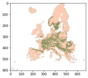
…and PNG thumbnails:
[7]:
thumb_fn = './stac_demo/odse/veg_fagus.sylvatica_anv.eml/veg_fagus.sylvatica_anv.eml_2018.01.01..2020.12.31/veg_fagus.sylvatica_anv.eml_p_30m_0..0cm_2018..2020_eumap_epsg3035_v0.2.png'
img = plt.imread(thumb_fn)
plt.imshow(img)
plt.show()
10.2. Accessing the catalog
We recommend also pystac to access our catalog:
[8]:
STAC_URL = 'https://s3.eu-central-1.wasabisys.com/stac/odse/catalog.json'
catalog = pystac.Catalog.from_file(STAC_URL)
Considering that the current implementation is a static catalog, without the search endpoint, we developed local STAC index, based on whoosh, to allow the users search for specific layers. The eumap.datasets.eo.STACIndex class can be used to provide similar functionality for any other static catalog compatible with STAC.
[9]:
index = STACIndex(catalog, verbose=True)
[23:57:42] Retriving all collections from OpenDataScience Europe
[23:58:02] Creating index for 184 collections
By default the local index is created in ./stac_index and after that you can execute full-text searches:
[10]:
result = index.search('Soil*')
print(json.dumps(result, sort_keys=True, indent=4))
[
    {
        "id": "sol_clay.tot.psa_eumap",
        "pos": 0,
        "title": "Soil clay content (2000\u20132020)"
    },
    {
        "id": "sol_db.od_eumap",
        "pos": 1,
        "title": "Soil bulk density (2000\u20132020)"
    },
    {
        "id": "sol_ph.h2o_eumap",
        "pos": 2,
        "title": "Soil pH in H2O (2000\u20132020)"
    },
    {
        "id": "sol_sand.tot.psa_eumap",
        "pos": 3,
        "title": "Soil sand content (2000\u20132020)"
    },
    {
        "id": "sol_log.oc_eumap",
        "pos": 4,
        "title": "Soil log organic carbon content (2000\u20132020)"
    }
]
Let’ use the search result to retrieve a collection by id and get its first item:
[11]:
collection_id = result[4]['id']
collection_first_item = next(catalog.get_child(collection_id).get_all_items())
collection_first_item
[11]:
<Item id=sol_log.oc_eumap_2000.01.01..2003.12.31>
For the returned item, let’s access all its assets.
You can access the same item in STAC-Browser to cross-check the result:
[12]:
 for key, item in collection_first_item.get_assets().items():
    print(f'- {key}:\n  {item}')
- log.oc_m_s0..0cm:
  <Asset href=https://s3.eu-central-1.wasabisys.com/eumap/sol/sol_log.oc_lucas.iso.10694_m_30m_s0..0cm_2000_eumap_epsg3035_v0.2.tif>
- log.oc_m_s30..30cm:
  <Asset href=https://s3.eu-central-1.wasabisys.com/eumap/sol/sol_log.oc_lucas.iso.10694_m_30m_s30..30cm_2000_eumap_epsg3035_v0.2.tif>
- log.oc_m_s60..60cm:
  <Asset href=https://s3.eu-central-1.wasabisys.com/eumap/sol/sol_log.oc_lucas.iso.10694_m_30m_s60..60cm_2000_eumap_epsg3035_v0.2.tif>
- log.oc_m_s100..100cm:
  <Asset href=https://s3.eu-central-1.wasabisys.com/eumap/sol/sol_log.oc_lucas.iso.10694_m_30m_s100..100cm_2000_eumap_epsg3035_v0.2.tif>
- log.oc_md_s0..0cm:
  <Asset href=https://s3.eu-central-1.wasabisys.com/eumap/sol/sol_log.oc_lucas.iso.10694_md_30m_s0..0cm_2000_eumap_epsg3035_v0.2.tif>
- log.oc_md_s30..30cm:
  <Asset href=https://s3.eu-central-1.wasabisys.com/eumap/sol/sol_log.oc_lucas.iso.10694_md_30m_s30..30cm_2000_eumap_epsg3035_v0.2.tif>
- log.oc_md_s60..60cm:
  <Asset href=https://s3.eu-central-1.wasabisys.com/eumap/sol/sol_log.oc_lucas.iso.10694_md_30m_s60..60cm_2000_eumap_epsg3035_v0.2.tif>
- log.oc_md_s100..100cm:
  <Asset href=https://s3.eu-central-1.wasabisys.com/eumap/sol/sol_log.oc_lucas.iso.10694_md_30m_s100..100cm_2000_eumap_epsg3035_v0.2.tif>
- thumbnail:
  <Asset href=https://s3.eu-central-1.wasabisys.com/stac/odse/sol_log.oc_eumap/sol_log.oc_eumap_2000.01.01..2003.12.31/sol_log.oc_lucas.iso.10694_m_30m_s0..0cm_2000_eumap_epsg3035_v0.2.png>
- log.oc_m_s30..30cm_preview:
  <Asset href=https://s3.eu-central-1.wasabisys.com/stac/odse/sol_log.oc_eumap/sol_log.oc_eumap_2000.01.01..2003.12.31/sol_log.oc_lucas.iso.10694_m_30m_s30..30cm_2000_eumap_epsg3035_v0.2.png>
- log.oc_m_s60..60cm_preview:
  <Asset href=https://s3.eu-central-1.wasabisys.com/stac/odse/sol_log.oc_eumap/sol_log.oc_eumap_2000.01.01..2003.12.31/sol_log.oc_lucas.iso.10694_m_30m_s60..60cm_2000_eumap_epsg3035_v0.2.png>
- log.oc_m_s100..100cm_preview:
  <Asset href=https://s3.eu-central-1.wasabisys.com/stac/odse/sol_log.oc_eumap/sol_log.oc_eumap_2000.01.01..2003.12.31/sol_log.oc_lucas.iso.10694_m_30m_s100..100cm_2000_eumap_epsg3035_v0.2.png>
- log.oc_md_s0..0cm_preview:
  <Asset href=https://s3.eu-central-1.wasabisys.com/stac/odse/sol_log.oc_eumap/sol_log.oc_eumap_2000.01.01..2003.12.31/sol_log.oc_lucas.iso.10694_md_30m_s0..0cm_2000_eumap_epsg3035_v0.2.png>
- log.oc_md_s30..30cm_preview:
  <Asset href=https://s3.eu-central-1.wasabisys.com/stac/odse/sol_log.oc_eumap/sol_log.oc_eumap_2000.01.01..2003.12.31/sol_log.oc_lucas.iso.10694_md_30m_s30..30cm_2000_eumap_epsg3035_v0.2.png>
- log.oc_md_s60..60cm_preview:
  <Asset href=https://s3.eu-central-1.wasabisys.com/stac/odse/sol_log.oc_eumap/sol_log.oc_eumap_2000.01.01..2003.12.31/sol_log.oc_lucas.iso.10694_md_30m_s60..60cm_2000_eumap_epsg3035_v0.2.png>
- log.oc_md_s100..100cm_preview:
  <Asset href=https://s3.eu-central-1.wasabisys.com/stac/odse/sol_log.oc_eumap/sol_log.oc_eumap_2000.01.01..2003.12.31/sol_log.oc_lucas.iso.10694_md_30m_s100..100cm_2000_eumap_epsg3035_v0.2.png>
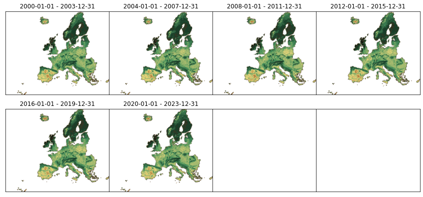
Let’s visualize all the thumbnails for the main asset:
[13]:
plot_stac_collection(catalog.get_child(collection_id))
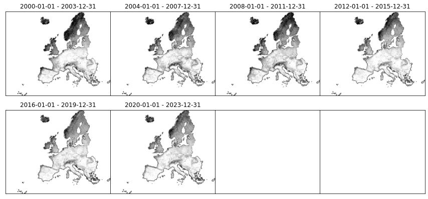
It’s also possible visualize thumbnails for a different asset informing the thumb_id:
[14]:
plot_stac_collection(catalog.get_child(collection_id), thumb_id='log.oc_md_s60..60cm_preview')
10.2.1. Data access and download
Now, we can retrieve all COG URLs for a specific asset (href property), what will allow us to read the actual raster data, as Numpy array, and later save it as local GeoTIFF files.
[15]:
def cog_urls(collection, asset_id):
    return [ item.assets[asset_id].href for item in collection.get_all_items() ]

collection_urls = cog_urls(catalog.get_child(collection_id), 'log.oc_m_s0..0cm')
print(json.dumps(collection_urls, sort_keys=True, indent=4))
[
    "https://s3.eu-central-1.wasabisys.com/eumap/sol/sol_log.oc_lucas.iso.10694_m_30m_s0..0cm_2000_eumap_epsg3035_v0.2.tif",
    "https://s3.eu-central-1.wasabisys.com/eumap/sol/sol_log.oc_lucas.iso.10694_m_30m_s0..0cm_2004_eumap_epsg3035_v0.2.tif",
    "https://s3.eu-central-1.wasabisys.com/eumap/sol/sol_log.oc_lucas.iso.10694_m_30m_s0..0cm_2008_eumap_epsg3035_v0.2.tif",
    "https://s3.eu-central-1.wasabisys.com/eumap/sol/sol_log.oc_lucas.iso.10694_m_30m_s0..0cm_2012_eumap_epsg3035_v0.2.tif",
    "https://s3.eu-central-1.wasabisys.com/eumap/sol/sol_log.oc_lucas.iso.10694_m_30m_s0..0cm_2016_eumap_epsg3035_v0.2.tif",
    "https://s3.eu-central-1.wasabisys.com/eumap/sol/sol_log.oc_lucas.iso.10694_m_30m_s0..0cm_2020_eumap_epsg3035_v0.2.tif"
]
As example, let’s use the bounding box of Wageningen / NL.
For a more interactively example, based on ipyleaflet, access ODSE Workshop 2021 - Training Sessions.
[16]:
bounds = (5.437546, 51.920556, 5.772629, 52.063468)
Let’s transform the bounding box to ETRS89/LAEA projection system before we can define a window to read the COG files:
[17]:
base_raster = rasterio.open(collection_urls[0])

transformer = Transformer.from_crs("epsg:4326", base_raster.crs, always_xy=True)
left, bottom = transformer.transform(bounds[0], bounds[1])
right, top = transformer.transform(bounds[2], bounds[3])

window = from_bounds(left, bottom, right, top, base_raster.transform)
print(f'left={left}, bottom={bottom}, right={right}, top={top}\n')
print(f'window = {window}')
left=4007342.4750108747, bottom=3210978.832030329, right=4031270.870186194, top=3225468.6391858133

window = Window(col_off=103578.08250036248, row_off=74484.71202713957, width=797.6131725106388, height=482.99357184948167)
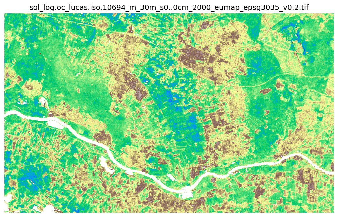
Using this window we can quickly read directly from a large COG file stored in our ODSE STAC.
[18]:
cog_url = collection_urls[0]

data, _ = read_rasters(raster_files=collection_urls, spatial_win=window, verbose=True)
plot_rasters(data[:,:,0].astype('float32'), cmaps="terrain_r", nodata=base_raster.nodata, titles=[ Path(cog_url).name ])
[23:58:08] Reading 6 raster files using 4 workers
Using eumap.raster.save_rasters we can save the clipped data by passing the COG as the reference file along with the window definition.
[19]:
roi_label = 'Wageningen'
workdir = Path('stac_download')

fn_rasters = [ workdir.joinpath(collection_id).joinpath(roi_label).joinpath(Path(url).name) for url in collection_urls ]
fn_rasters = save_rasters(fn_base_raster=collection_urls[0], fn_raster_list=fn_rasters, data=data, spatial_win=window, verbose=True)

print(json.dumps([str(f) for f in fn_rasters], sort_keys=True, indent=4))
[23:58:12] Writing 6 raster files using 4 workers
[
    "stac_download/sol_log.oc_eumap/Wageningen/sol_log.oc_lucas.iso.10694_m_30m_s0..0cm_2000_eumap_epsg3035_v0.2.tif",
    "stac_download/sol_log.oc_eumap/Wageningen/sol_log.oc_lucas.iso.10694_m_30m_s0..0cm_2004_eumap_epsg3035_v0.2.tif",
    "stac_download/sol_log.oc_eumap/Wageningen/sol_log.oc_lucas.iso.10694_m_30m_s0..0cm_2008_eumap_epsg3035_v0.2.tif",
    "stac_download/sol_log.oc_eumap/Wageningen/sol_log.oc_lucas.iso.10694_m_30m_s0..0cm_2012_eumap_epsg3035_v0.2.tif",
    "stac_download/sol_log.oc_eumap/Wageningen/sol_log.oc_lucas.iso.10694_m_30m_s0..0cm_2016_eumap_epsg3035_v0.2.tif",
    "stac_download/sol_log.oc_eumap/Wageningen/sol_log.oc_lucas.iso.10694_m_30m_s0..0cm_2020_eumap_epsg3035_v0.2.tif"
]